Data Engineering with Arrow

Data Engineering

https://en.wikipedia.org/wiki/Data_engineering

.NORM Files

https://xkcd.com/2116/

Poll: Formats

Which file formats do you use most often?

• 1️⃣ CSV (.csv)
• 2️⃣ MS Excel (.xls and .xlsx)
• 3️⃣ Parquet (.parquet)
• 4️⃣ Something else

Arrow & File Formats

Seattle
Checkouts
Big CSV

https://data.seattle.gov/Community/Checkouts-by-Title/tmmm-ytt6

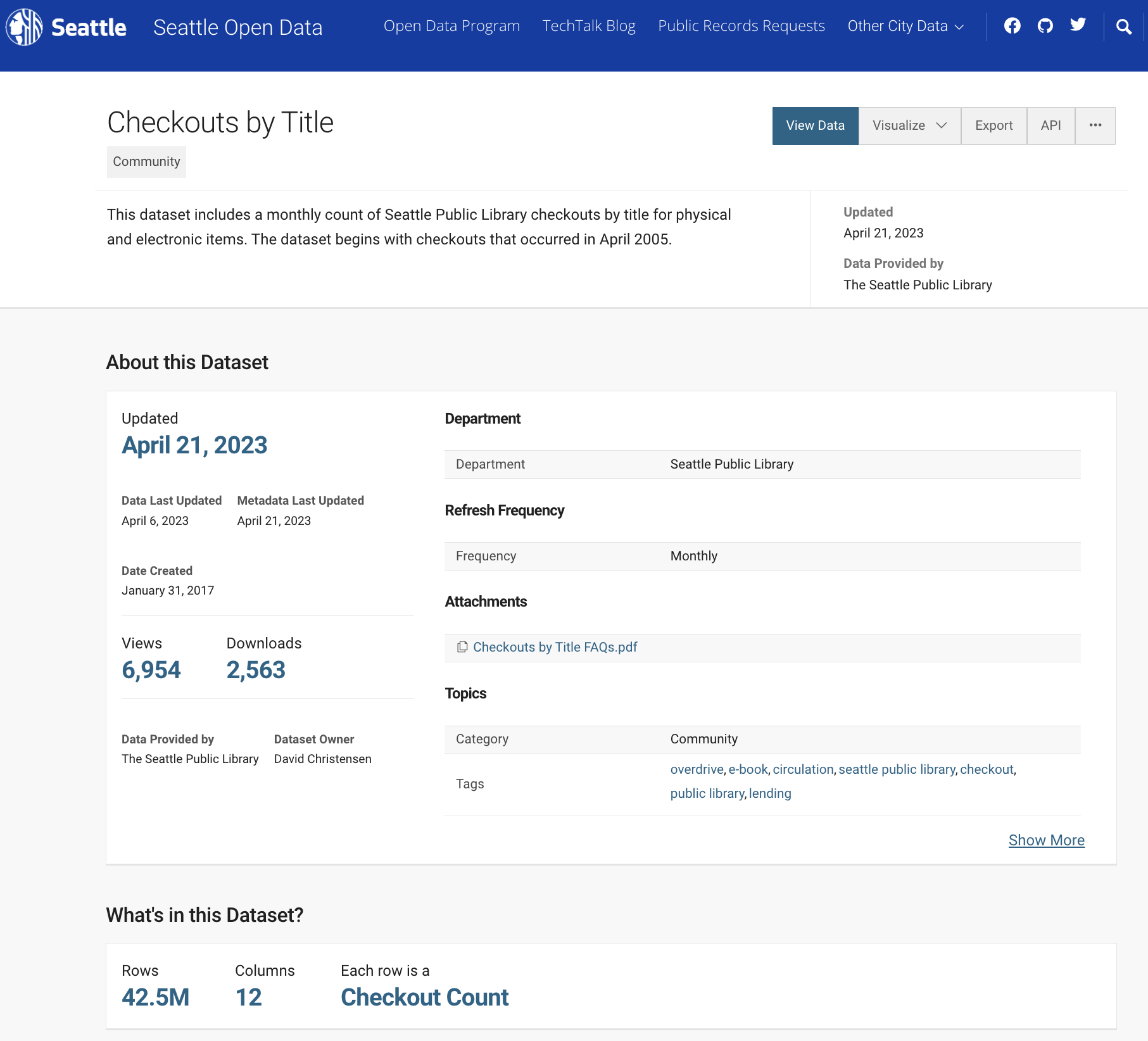
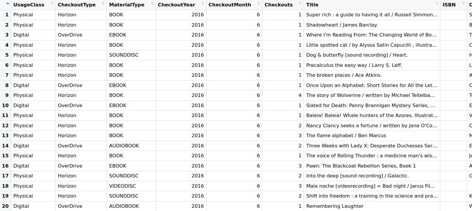
Dataset contents

arrow::open_dataset() with a CSV

library(arrow)
library(dplyr)

seattle_csv <- open_dataset(sources = "data/seattle-library-checkouts.csv",
                            format = "csv")
seattle_csv

FileSystemDataset with 1 csv file
12 columns
UsageClass: string
CheckoutType: string
MaterialType: string
CheckoutYear: int64
CheckoutMonth: int64
Checkouts: int64
Title: string
ISBN: null
Creator: string
Subjects: string
Publisher: string
PublicationYear: string

Arrow Data Types

Arrow has a rich data type system, including direct analogs of many R data types

• <dbl> == <double>
• <chr> == <string> OR <utf8> (aliases)
• <int> == <int32>

https://arrow.apache.org/docs/r/articles/data_types.html

arrow::schema()

Create a schema or extract one from an object.

Let’s extract the schema:

schema(seattle_csv)

Schema
UsageClass: string
CheckoutType: string
MaterialType: string
CheckoutYear: int64
CheckoutMonth: int64
Checkouts: int64
Title: string
ISBN: null
Creator: string
Subjects: string
Publisher: string
PublicationYear: string

Parsing the Metadata

Arrow scans 👀 1MB of data to impute or “guess” the data types

📚 arrow vs readr blog post: https://thisisnic.github.io/2022/11/21/type-inference-in-readr-and-arrow/

Parsers Are Not Always Right

schema(seattle_csv)

Schema
UsageClass: string
CheckoutType: string
MaterialType: string
CheckoutYear: int64
CheckoutMonth: int64
Checkouts: int64
Title: string
ISBN: null
Creator: string
Subjects: string
Publisher: string
PublicationYear: string

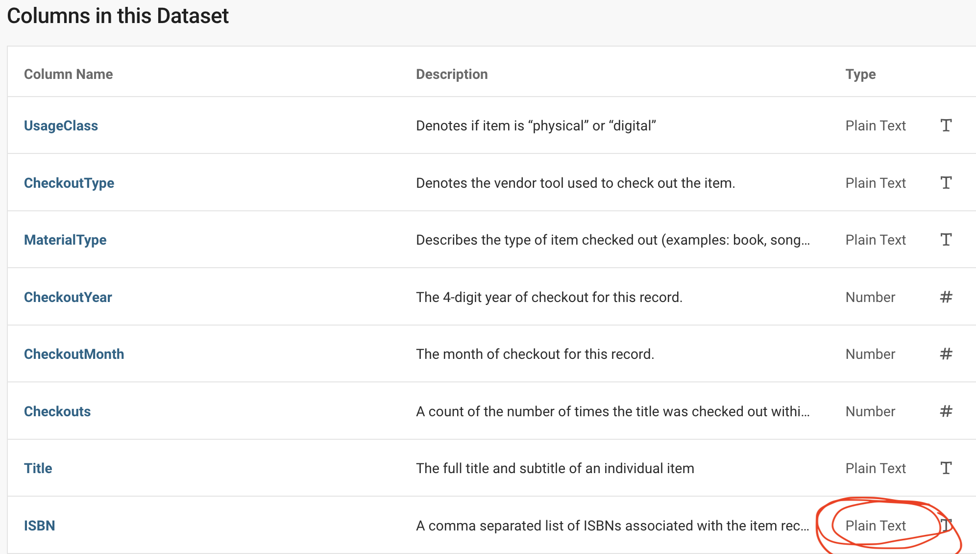
International Standard Book Number (ISBN) is a 13-digit number that uniquely identifies books and book-like products published internationally.

Data Dictionaries, metadata in data catalogues should provide this info.

The number or rows used to infer the schema will vary depending on the data in each column, total number of columns, and how many bytes each value takes up in memory.

If all of the values in a column that lie within the first 1MB of the file are missing values, arrow will classify this data as null type. ISBN! Phone numbers, zip codes, leading zeros…

Recommended specifying a schema when working with CSV datasets to avoid potential issues like this

Let’s Control the Schema

Creating a schema manually:

schema(
  UsageClass = utf8(),
  CheckoutType = utf8(),
  MaterialType = utf8(),
  CheckoutYear = int64(),
  CheckoutMonth = int64(),
  Checkouts = int64(),
  Title = utf8(),
  ISBN = string(), #utf8()
  Creator = utf8(),
  Subjects = utf8(),
  Publisher = utf8(),
  PublicationYear = utf8()
)

This will take a lot of typing with 12 columns 😢

Let’s Control the Schema

Use the code() method to extract the code from the schema:

seattle_csv$schema$code() 

schema(UsageClass = utf8(), CheckoutType = utf8(), MaterialType = utf8(), 
    CheckoutYear = int64(), CheckoutMonth = int64(), Checkouts = int64(), 
    Title = utf8(), ISBN = null(), Creator = utf8(), Subjects = utf8(), 
    Publisher = utf8(), PublicationYear = utf8())

🤩

Let’s Control the Schema

Schema defines column names and types, so we need to skip the first row (skip = 1):

seattle_csv <- open_dataset(sources = "data/seattle-library-checkouts.csv",
  format = "csv",
  schema = schema(
    UsageClass = utf8(),
    CheckoutType = utf8(),
    MaterialType = utf8(),
    CheckoutYear = int64(),
    CheckoutMonth = int64(),
    Checkouts = int64(),
    Title = utf8(),
    ISBN = string(), #utf8()
    Creator = utf8(),
    Subjects = utf8(),
    Publisher = utf8(),
    PublicationYear = utf8()
  ),
    skip = 1,
)
seattle_csv

FileSystemDataset with 1 csv file
12 columns
UsageClass: string
CheckoutType: string
MaterialType: string
CheckoutYear: int64
CheckoutMonth: int64
Checkouts: int64
Title: string
ISBN: string
Creator: string
Subjects: string
Publisher: string
PublicationYear: string

Let’s Control the Schema

Supply column types for a subset of columns by providing a partial schema:

seattle_csv <- open_dataset(
  sources = "data/seattle-library-checkouts.csv",
  format = "csv",
  col_types = schema(ISBN = string()) #utf8()
)
seattle_csv

FileSystemDataset with 1 csv file
12 columns
UsageClass: string
CheckoutType: string
MaterialType: string
CheckoutYear: int64
CheckoutMonth: int64
Checkouts: int64
Title: string
ISBN: string
Creator: string
Subjects: string
Publisher: string
PublicationYear: string

Your Turn

1. The first few thousand rows of ISBN are blank in the Seattle Checkouts CSV file. Read in the Seattle Checkouts CSV file with open_dataset() and ensure the correct data type for ISBN is <string> (or the alias <utf8>) instead of the <null> interpreted by Arrow.

2. Once you have a Dataset object with the correct data types, count the number of Checkouts by CheckoutYear and arrange the result by CheckoutYear.

➡️ Data Storage Engineering Exercises Page

9GB CSV file + arrow + dplyr

seattle_csv |>
  group_by(CheckoutYear) |>
  summarise(sum(Checkouts)) |>
  arrange(CheckoutYear) |> 
  collect()

# A tibble: 18 × 2
   CheckoutYear `sum(Checkouts)`
          <int>            <int>
 1         2005          3798685
 2         2006          6599318
 3         2007          7126627
 4         2008          8438486
 5         2009          9135167
 6         2010          8608966
 7         2011          8321732
 8         2012          8163046
 9         2013          9057096
10         2014          9136081
11         2015          9084179
12         2016          9021051
13         2017          9231648
14         2018          9149176
15         2019          9199083
16         2020          6053717
17         2021          7361031
18         2022          7001989

9GB CSV file + arrow + dplyr

seattle_csv |>
  group_by(CheckoutYear) |>
  summarise(sum(Checkouts)) |>
  arrange(CheckoutYear) |> 
  collect() |>
  system.time()

   user  system elapsed 
 10.615   1.253  10.356 

42 million rows – not bad, but could be faster….

File Format: Apache Parquet

https://parquet.apache.org/

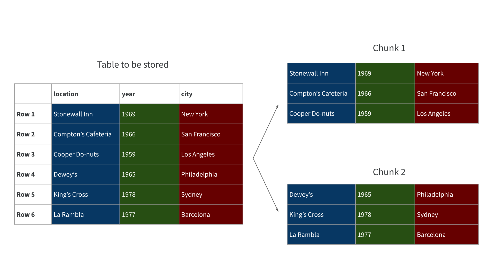
Parquet Files: “row-chunked”

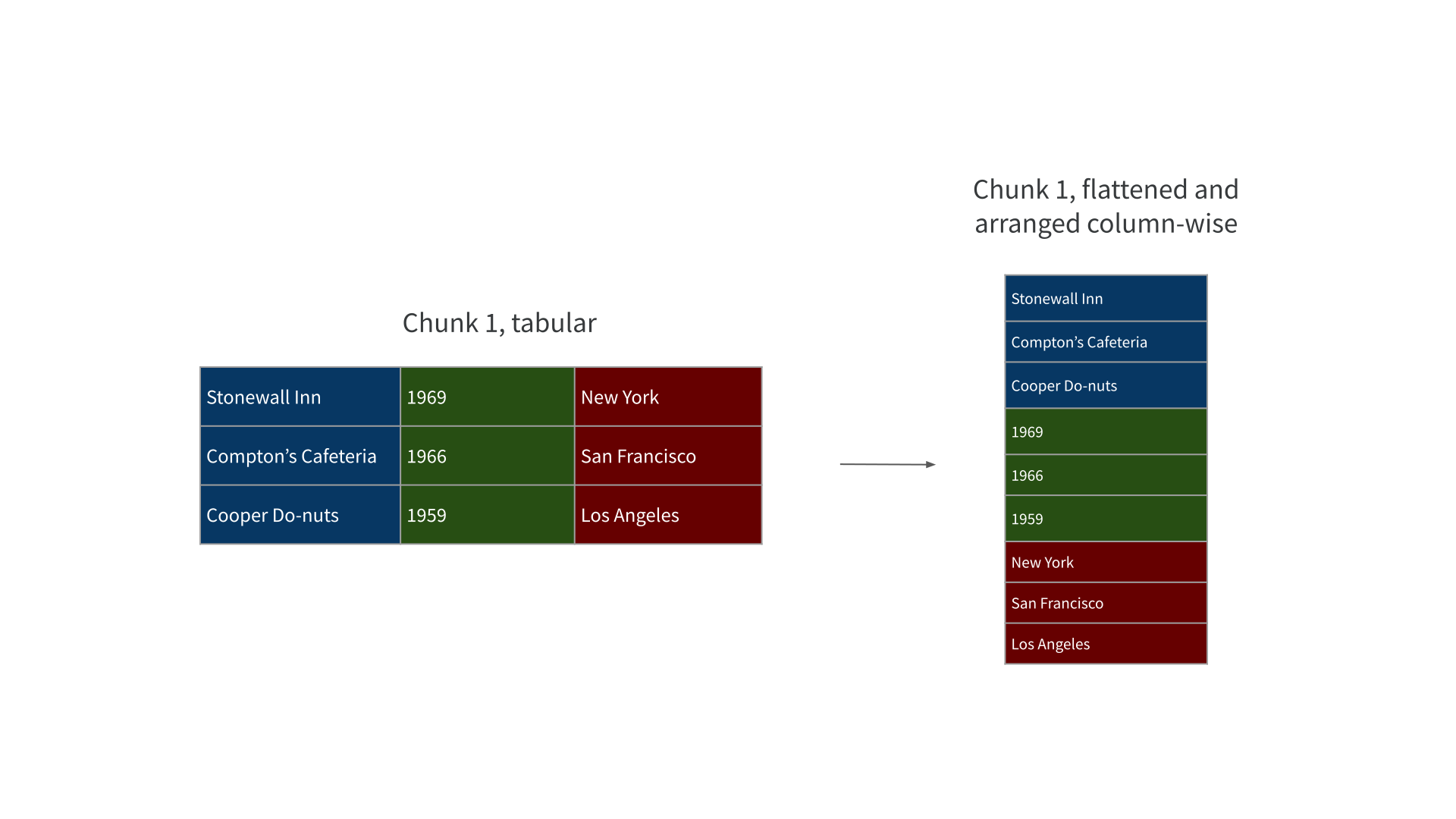
Parquet Files: “row-chunked & column-oriented”

Parquet

• “row-chunked & column-oriented” == work on different parts of the file at the same time or skip some chunks all together, better performance than row-by-row
• compression and encoding == usually much smaller than equivalent CSV file, less data to move from disk to memory
• rich type system & stores the schema along with the data == more robust pipelines

• efficient encodings to keep file size down, and supports file compression, less data to move from disk to memory
• CSV has no info about data types, inferred by each parser

Writing to Parquet

seattle_parquet <- "data/seattle-library-checkouts-parquet"

seattle_csv |>
  write_dataset(path = seattle_parquet,
                format = "parquet")

Storage: Parquet vs CSV

file <- list.files(seattle_parquet)
file.size(file.path(seattle_parquet, file)) / 10**9

[1] 4.424267

Parquet about half the size of the CSV file on-disk 💾

Your Turn

1. Re-run the query counting the number of Checkouts by CheckoutYear and arranging the result by CheckoutYear, this time using the Seattle Checkout data saved to disk as a single Parquet file. Did you notice a difference in compute time?

➡️ Data Storage Engineering Exercises Page

4.5GB Parquet file + arrow + dplyr

open_dataset(sources = seattle_parquet, 
             format = "parquet") |>
  group_by(CheckoutYear) |>
  summarise(sum(Checkouts)) |>
  arrange(CheckoutYear) |> 
  collect() |>
  system.time()

   user  system elapsed 
  1.744   0.427   0.594 

42 million rows – much better! But could be even faster….

File Storage:
Partitioning

Dividing data into smaller pieces, making it more easily accessible and manageable

also called multi-files or sometimes shards

Poll: Partitioning?

Have you partitioned your data or used partitioned data before today?

• 1️⃣ Yes
• 2️⃣ No
• 3️⃣ Not sure, the data engineers sort that out!

Art & Science of Partitioning

• avoid files < 20MB and > 2GB
• avoid > 10,000 files (🤯)
• partition on variables used in filter()

• guidelines not rules, results vary
• experiment, especially with cloud
• arrow suggests avoid files smaller than 20MB and larger than 2GB
• avoid partitions that produce more than 10,000 files
• partition by variables that you filter by, allows arrow to only read relevant files

Rewriting the Data Again

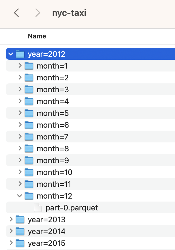
seattle_parquet_part <- "data/seattle-library-checkouts"

seattle_csv |>
  group_by(CheckoutYear) |>
  write_dataset(path = seattle_parquet_part,
                format = "parquet")

What Did We “Engineer”?

seattle_parquet_part <- "data/seattle-library-checkouts"

sizes <- tibble(
  files = list.files(seattle_parquet_part, recursive = TRUE),
  size_GB = file.size(file.path(seattle_parquet_part, files)) / 10**9
)

sizes

# A tibble: 18 × 2
   files                            size_GB
   <chr>                              <dbl>
 1 CheckoutYear=2005/part-0.parquet   0.115
 2 CheckoutYear=2006/part-0.parquet   0.172
 3 CheckoutYear=2007/part-0.parquet   0.186
 4 CheckoutYear=2008/part-0.parquet   0.204
 5 CheckoutYear=2009/part-0.parquet   0.224
 6 CheckoutYear=2010/part-0.parquet   0.233
 7 CheckoutYear=2011/part-0.parquet   0.250
 8 CheckoutYear=2012/part-0.parquet   0.261
 9 CheckoutYear=2013/part-0.parquet   0.282
10 CheckoutYear=2014/part-0.parquet   0.296
11 CheckoutYear=2015/part-0.parquet   0.308
12 CheckoutYear=2016/part-0.parquet   0.315
13 CheckoutYear=2017/part-0.parquet   0.319
14 CheckoutYear=2018/part-0.parquet   0.306
15 CheckoutYear=2019/part-0.parquet   0.303
16 CheckoutYear=2020/part-0.parquet   0.158
17 CheckoutYear=2021/part-0.parquet   0.240
18 CheckoutYear=2022/part-0.parquet   0.252

4.5GB partitioned Parquet files + arrow + dplyr

seattle_parquet_part <- "data/seattle-library-checkouts"

open_dataset(sources = seattle_parquet_part,
             format = "parquet") |>
  group_by(CheckoutYear) |>
  summarise(sum(Checkouts)) |>
  arrange(CheckoutYear) |> 
  collect() |>
  system.time()

   user  system elapsed 
  1.631   0.388   0.358 

42 million rows – not too shabby!

Your Turn

1. Let’s write the Seattle Checkout CSV data to a multi-file dataset just one more time! This time, write the data partitioned by CheckoutType as Parquet files.

2. Now compare the compute time between our Parquet data partitioned by CheckoutYear and our Parquet data partitioned by CheckoutType with a query of the total number of checkouts in September of 2019. Did you find a difference in compute time?

➡️ Data Storage Engineering Exercises Page

Partition Design

seattle_checkouttype <- "data/seattle-library-checkouts-type"

seattle_csv |>
  group_by(CheckoutType) |>
  write_dataset(path = seattle_checkouttype,
                format = "parquet")

Filter == Partition

open_dataset("data/seattle-library-checkouts") |> 
  filter(CheckoutYear == 2019, CheckoutMonth == 9) |> 
  summarise(TotalCheckouts = sum(Checkouts)) |>
  collect() |> 
  system.time()

   user  system elapsed 
  0.035   0.005   0.028 

Filter != Partition

open_dataset(sources = "data/seattle-library-checkouts-type") |> 
  filter(CheckoutYear == 2019, CheckoutMonth == 9) |> 
  summarise(TotalCheckouts = sum(Checkouts)) |>
  collect() |> 
  system.time()

   user  system elapsed 
  0.859   0.091   0.327 

Partition Design

• Partitioning on variables commonly used in filter() often faster
• Number of partitions also important (Arrow reads the metadata of each file)

Partitions & NA Values

Default:

partition_na_default_path <- "data/na-partition-default"

write_dataset(starwars,
              partition_na_default_path,
              partitioning = "hair_color")

list.files(partition_na_default_path)

 [1] "hair_color=__HIVE_DEFAULT_PARTITION__"
 [2] "hair_color=auburn"                    
 [3] "hair_color=auburn%2C%20grey"          
 [4] "hair_color=auburn%2C%20white"         
 [5] "hair_color=black"                     
 [6] "hair_color=blond"                     
 [7] "hair_color=blonde"                    
 [8] "hair_color=brown"                     
 [9] "hair_color=brown%2C%20grey"           
[10] "hair_color=grey"                      
[11] "hair_color=none"                      
[12] "hair_color=white"                     

Partitions & NA Values

Custom:

partition_na_custom_path <- "data/na-partition-custom"

write_dataset(starwars,
              partition_na_custom_path,
              partitioning = hive_partition(hair_color = string(),
                                            null_fallback = "no_color"))

list.files(partition_na_custom_path)

 [1] "hair_color=auburn"            "hair_color=auburn%2C%20grey" 
 [3] "hair_color=auburn%2C%20white" "hair_color=black"            
 [5] "hair_color=blond"             "hair_color=blonde"           
 [7] "hair_color=brown"             "hair_color=brown%2C%20grey"  
 [9] "hair_color=grey"              "hair_color=no_color"         
[11] "hair_color=none"              "hair_color=white"            

Performance Review: Single CSV

How long does it take to calculate the number of books checked out in each month of 2021?

open_dataset(sources = "data/seattle-library-checkouts.csv", 
  format = "csv") |> 

  filter(CheckoutYear == 2021, MaterialType == "BOOK") |>
  group_by(CheckoutMonth) |>
  summarise(TotalCheckouts = sum(Checkouts)) |>
  collect() |>
  system.time()

   user  system elapsed 
 11.658   1.272  11.225 

Performance Review: Partitioned Parquet

How long does it take to calculate the number of books checked out in each month of 2021?

open_dataset(sources = "data/seattle-library-checkouts",
             format = "parquet") |> 
  filter(CheckoutYear == 2021, MaterialType == "BOOK") |>
  group_by(CheckoutMonth) |>
  summarise(TotalCheckouts = sum(Checkouts)) |>
  collect() |> 
  system.time()

   user  system elapsed 
  0.218   0.046   0.069 

Engineering Data Tips for Improved Storage & Performance

• consider “column-oriented” file formats like Parquet
• consider partitioning, experiment to get an appropriate partition design 🗂️
• watch your schemas 👀

R for Data Science (2e)

Chapter 23: Arrow

https://r4ds.hadley.nz/