con <- dbConnect(odbc::odbc(),
  Driver = ".../lib/libsparkodbc_sb64-universal.dylib",
  Host = Sys.getenv("DATABRICKS_HOST"),
  PWD = Sys.getenv("DATABRICKS_TOKEN"),
  HTTPPath = "/sql/1.0/warehouses/300bd24ba12adf8e",
  Port = 443,
  AuthMech = 3,
  Protocol = "https",
  ThriftTransport = 2,
  SSL = 1,
UID = "token")The team


Edgar Ruiz
Instructor
James Blair
TA
Posit + Databricks
Special work we have done as part of the new partnership

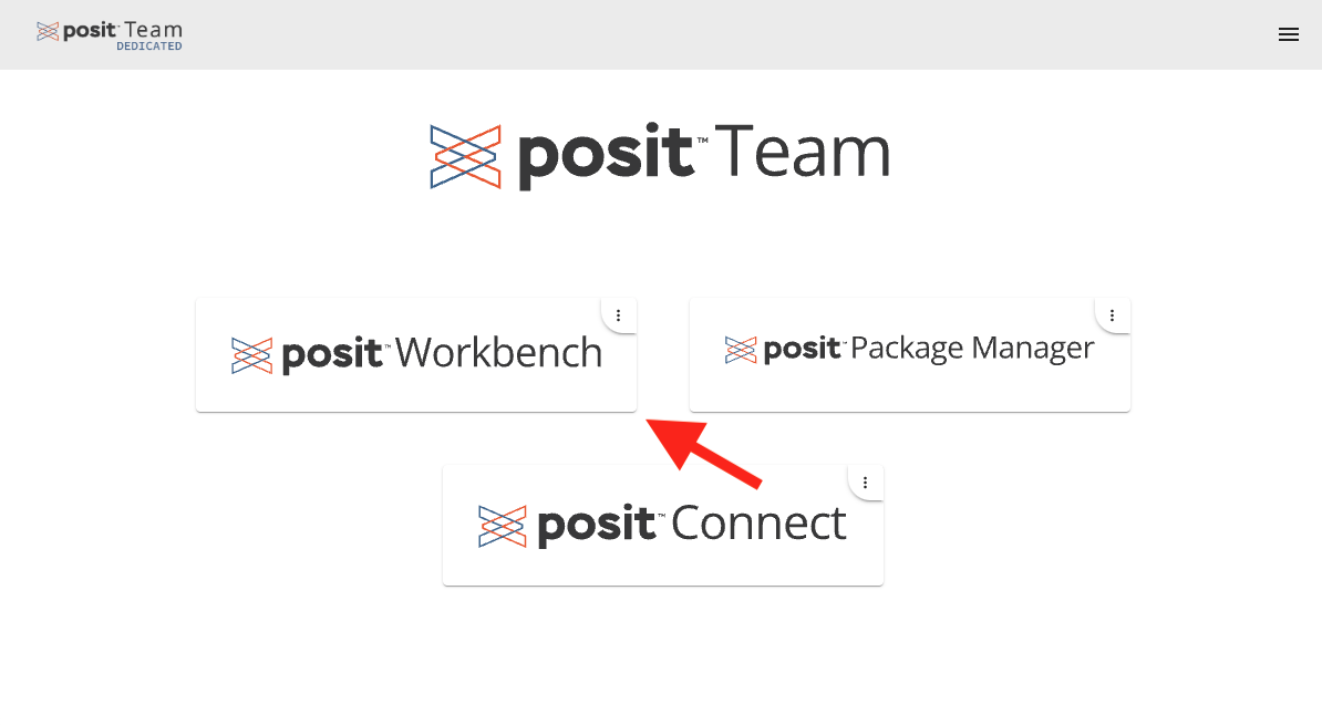
Step 1 - Landing Page
Navigate to conf.posit.team, click on Posit Workbench
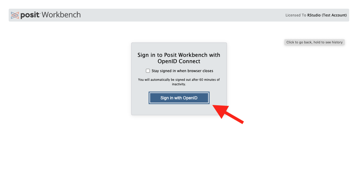
Step 2 - OpenID Page
Click on Sign in with OpenID
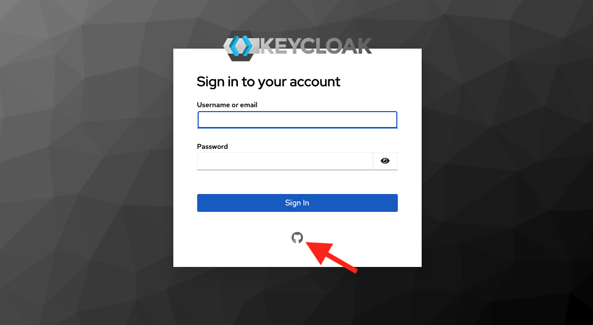
Step 3 - KeyCloak Page
Click on the GitHub icon
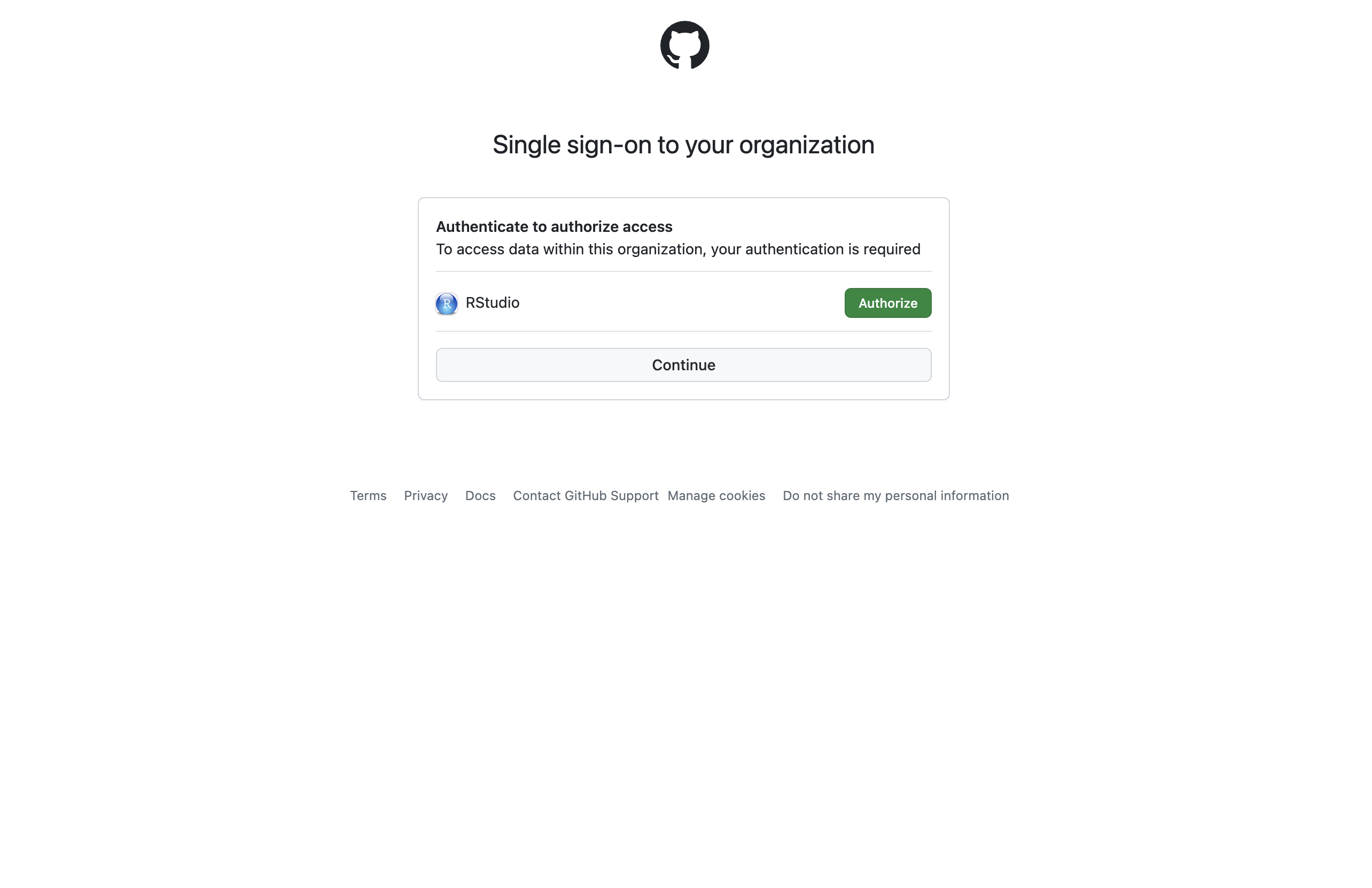
Step 4 - GitHub
Log into GitHub, and/or approve the RStudio org
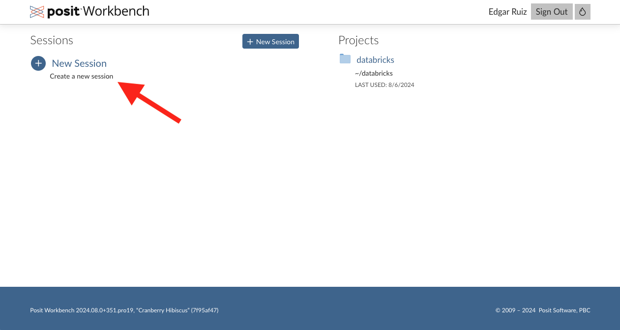
Step 5 - Posit Workbench homepage
Click on the New Session button
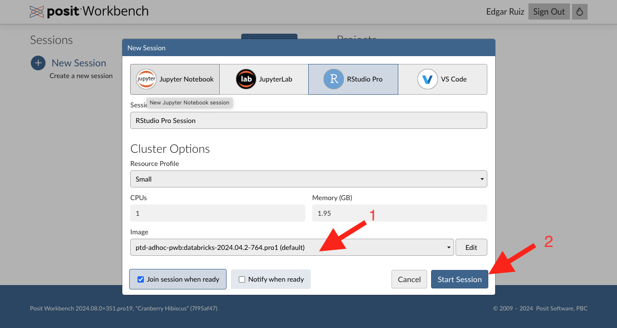
Step 6 - Setup new session
Confirm that the image matches what’s on the screenshot (1), then click on Start Session (2).
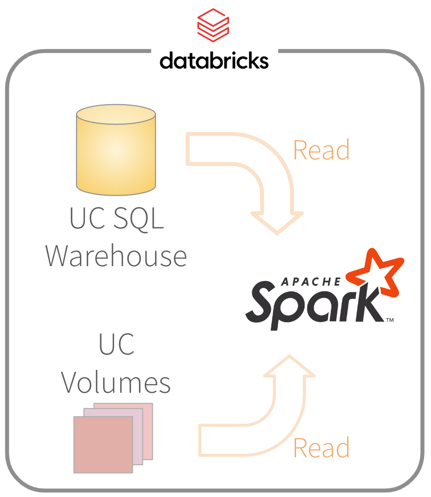
Working with Databricks
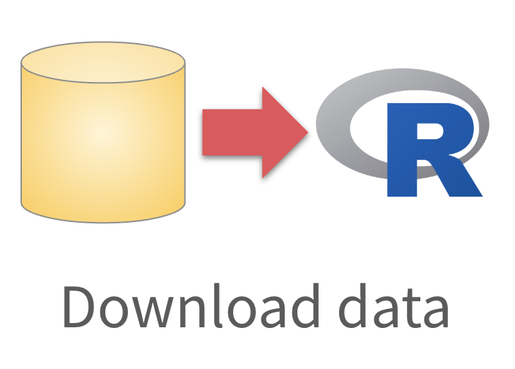
“Default” approach

“Default” approach
“Default” approach

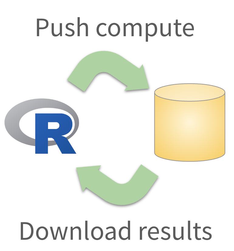
Better approach!
Better approach!
Better approach!
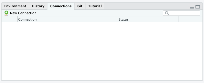
Using RStudio
In the “Connections” pane, select “New Connection”
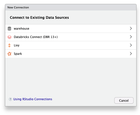
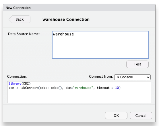
Using RStudio
Select ‘warehouse’
Using RStudio
Click ‘OK’
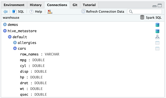
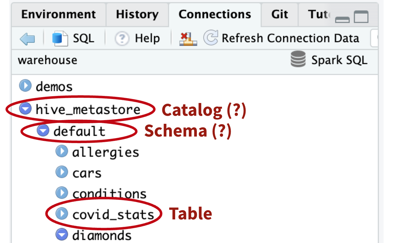
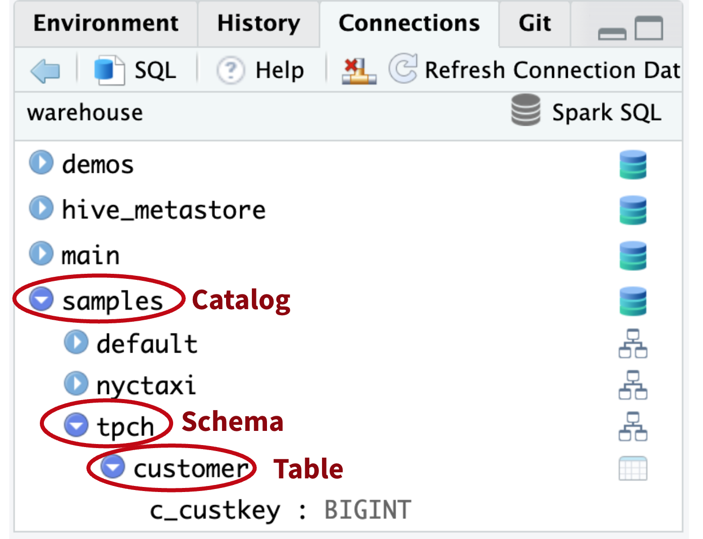
RStudio DB Navigator
Explore the catalogs, schema and tables
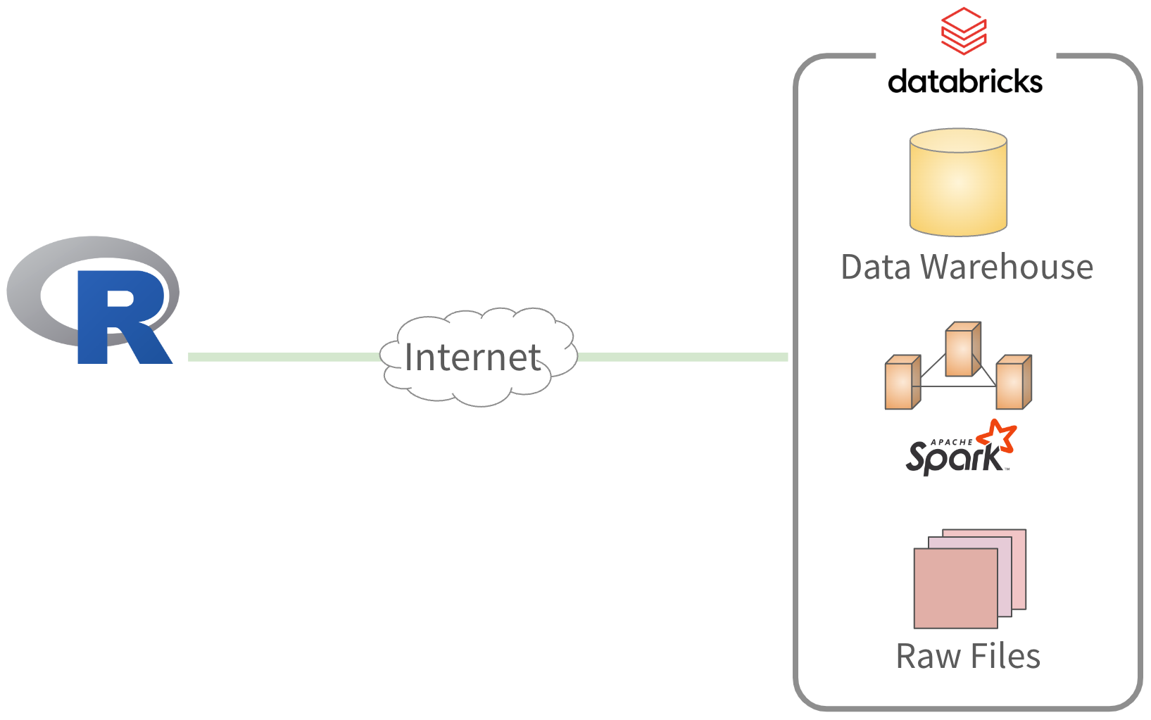
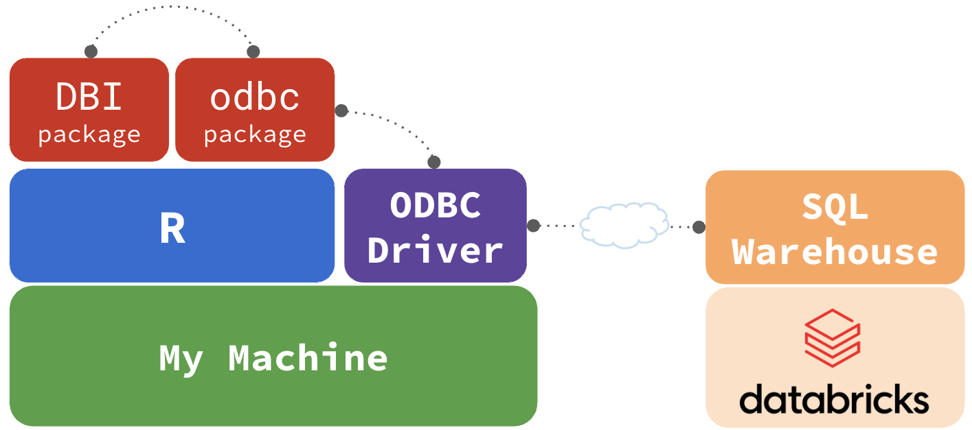
How everything connects
Connecting - Better
odbc::databricks()simplifies the setup- Automatically detects credentials, driver, and sets default arguments
HTTPPathis the only argument that you will need
con <- dbConnect(
  odbc::databricks(),
  HTTPPath = "/sql/1.0/warehouses/300bd24ba12adf8e"
)How everything connects (Revisited)
Other RStudio interfaces
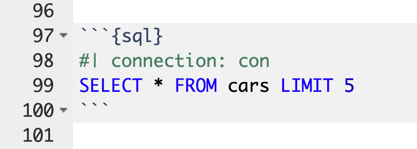
knitr SQL engine
RStudio SQL script
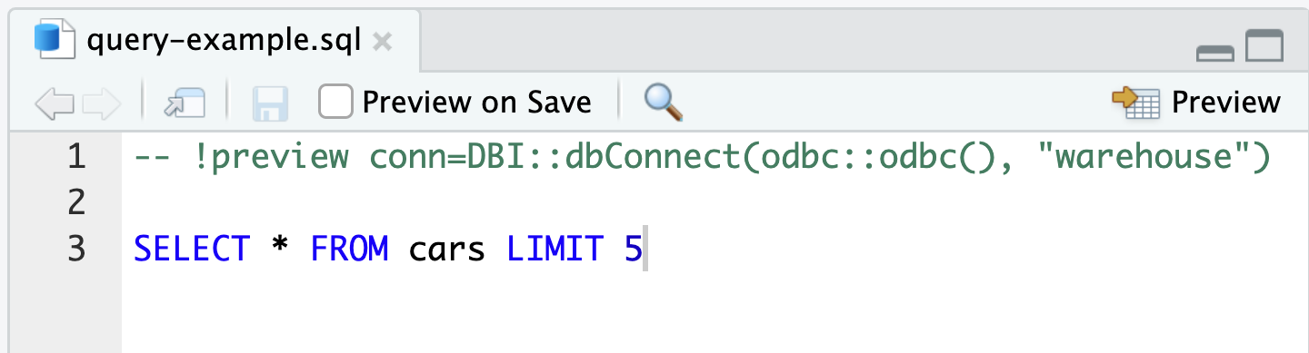
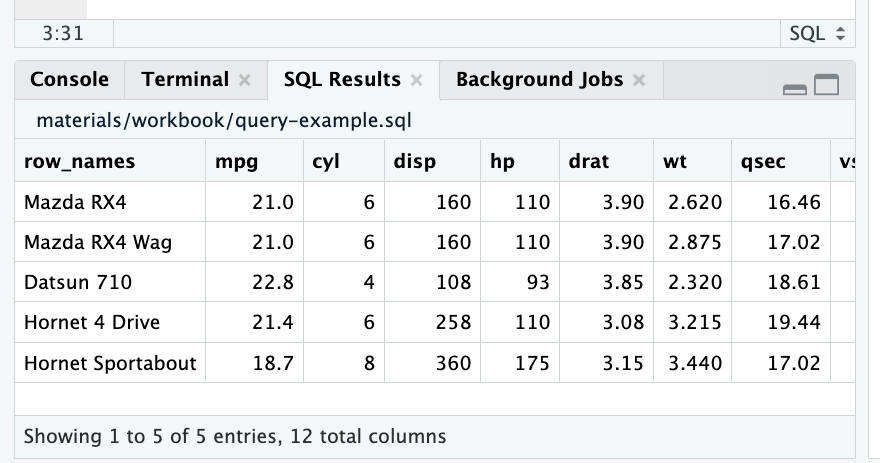
Approaches
Preferred
“Use in case of emergencies”
Use dplyr & dbplyr

- Translates R code to SQL!
- ‘Modularity’ of piped code
- Guardrails against pulling all of the data
- All your code is in R
tbl(con, "diamonds") |>
  group_by(cut) |>
  summarise(
    avg_price = mean(price, na.rm = TRUE)
  ) |>
  arrange(desc(avg_price))
🔑 How does it work?
- Creates a “virtual” table
- Behaves like a regular data frame
- It contains no data
- It’s a pointer to the database table
tbl_diamonds <- tbl(con, “diamonds”)

tbl_diamonds |>
  count()

Source: SQL [1 x 1]
Database: Spark SQL 3.1.1[token@Spark SQL/hive_metastore]
   n
<int64>
1 53940
🔑 How does it work?
- Create a variable in R without importing data
- SQL is sent only when data is requested
- Behind the scenes, translates code to SQL
tbl_diamonds |>
  count() |>
  show_query()

<SQL>
SELECT COUNT(*) AS ‘n’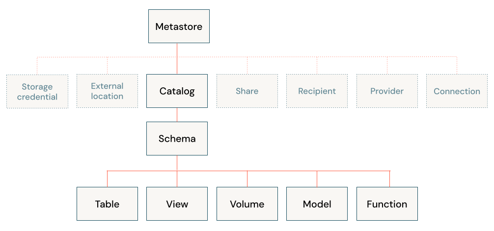
FROM ‘diamonds’Databricks Unity Catalog (UC)
Centralizes access control, auditing, lineage, and data discovery across workspaces.
Accessing the UC
“diamonds” can be accessed without specifying catalog and schema
# Why do you work?!
tbl(con, “diamonds”)
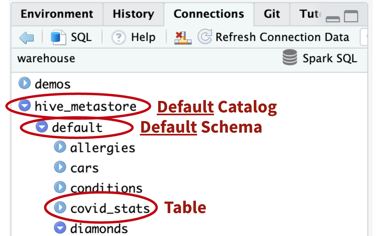
Accessing the UC
“hive_metastore” & “default” are the default catalog & schema respectively
# Oooh, that’s why!
tbl(con, “diamonds”)
Non-default catalog
How do I access tables not in the default catalog?
tbl(con, “customer”)
x (31740) Table or view not found: ..customer
Non-default catalog
How do I access tables not in the default catalog?
tbl(con, “customer”)
x (31740) Table or view not found: ..customer
tbl(
Xcon,
X“workshops.tpch.customer”
X)
x (31740) Table or view not found: ..workshops.tpch.
customer
Non-default catalog
Use I() to create the correct table reference
tbl(
Xcon,
XI(“workshops.tpch.customer”)
X)
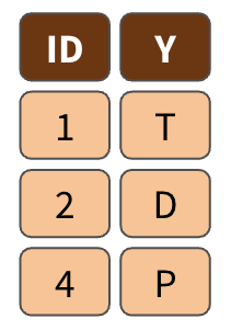
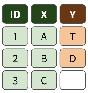
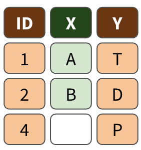
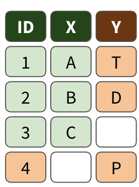
Joining tables
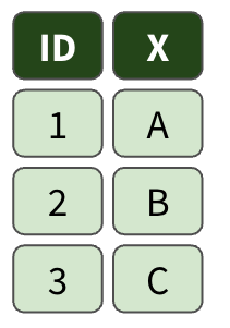
left_join()
right_join()
full_join()
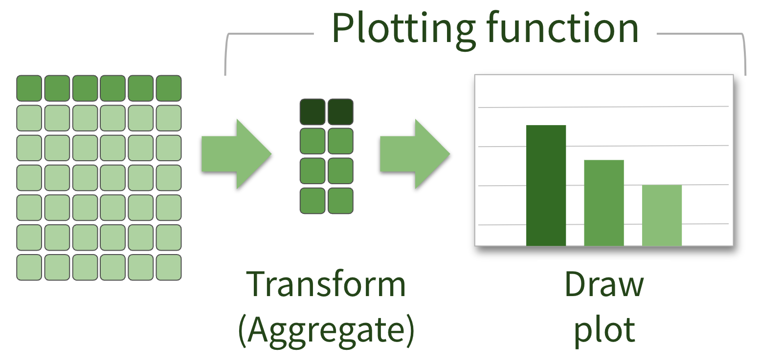
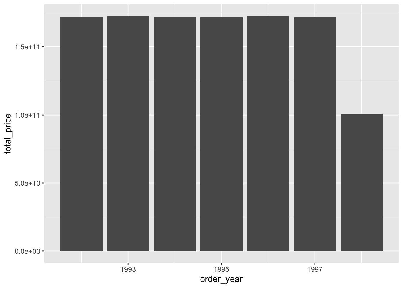
Plotting local data
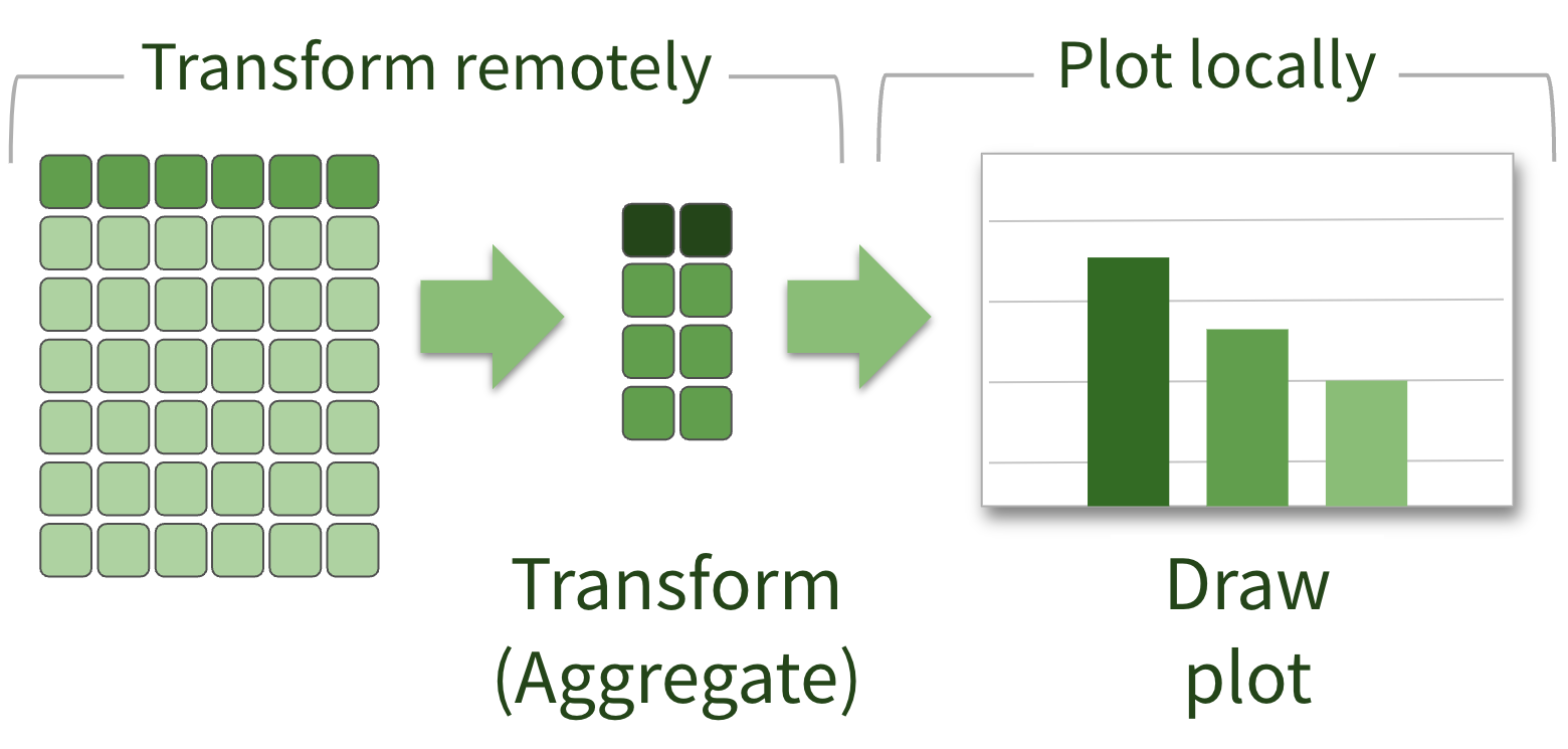
Plotting remote data
What that looks like in R
Pipe the prepared data into a ggplot2
What that looks like in R
Pipe the prepared data into a ggplot2
prep_orders |>
  group_by(order_year) |>
  summarise(
   total_price = sum(o_totalprice, na.rm = TRUE)
  ) |>
  arrange(order_year) |>
  ggplot() +
  geom_col(
    aes(order_year, total_price)
) 
What that looks like in R
Pipe the prepared data into a ggplot2
prep_orders |>
  group_by(order_year) |>
  summarise(
    total_price = sum(o_totalprice, na.rm = TRUE)
  ) |>
  collect() |> # Why are you missing?
  arrange(order_year) |>
  ggplot() +
  geom_col(aes(order_year, total_price))
ggplot2 “auto-collects”
Be careful! It downloads all of the data!
nation <- tbl(
  con,
  I("workshops.tpch.nation")
  )

nation |>
  ggplot() +
  geom_col(aes(n_name, n_regionkey))
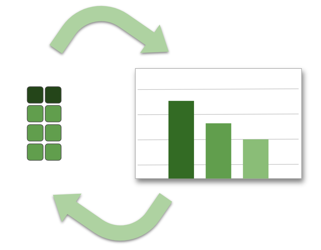
The truth about ggplot2
A plot gets refined iteratively, data must be local.
- ‘Improve scales’
- ‘Add labels to the data’
- ‘Add title and subtitle’
- ‘Improve colors’
- ‘Change the theme’
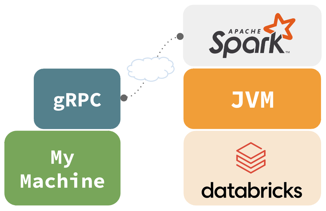
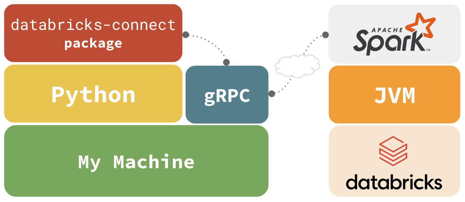
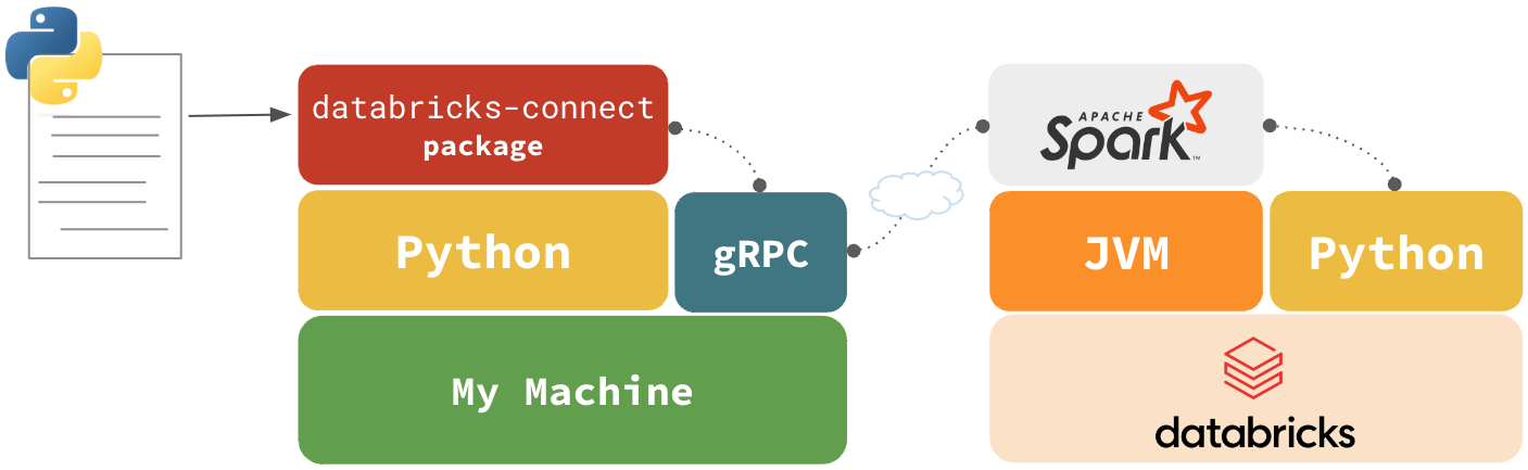
Databricks Connect
- Spark Connect, offers true remote connectivity
- Uses gRPC to as the communication interface
- Databricks Connect ‘v2’ is based on Spark Connect (DBR 13+)
Databricks Connect
databricks-connect integrates with gRPC via pyspark
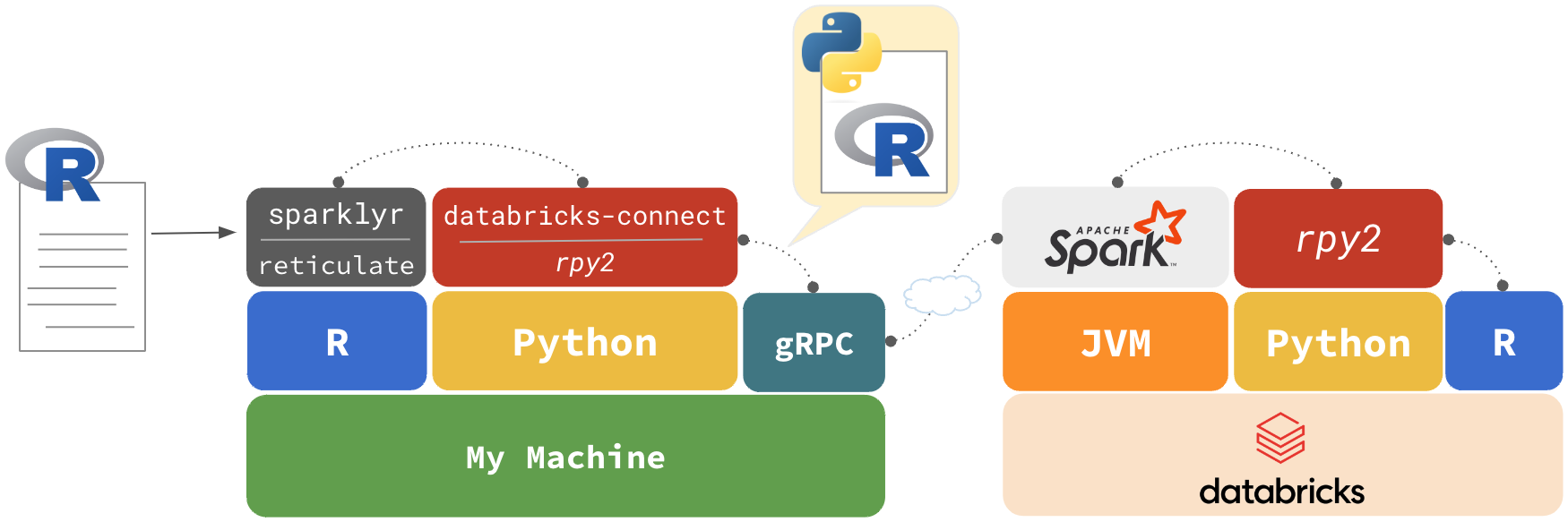
Databricks Connect
sparklyr integrates with databricks-connect via reticulate
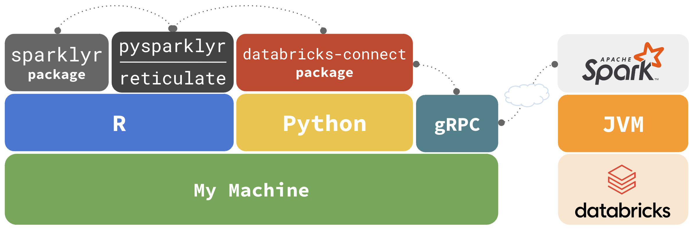
Why not just use ‘reticulate’?
sparklyr extends functionality and user experience
dplyrback-endDBIback-end- R UDFs
- RStudio, and Positron, Connections Pane integration
Getting started
- Python 3.10+
- A Python environment with
databricks-connectand its dependencies pysparklyrextension
install.packages("pysparklyr")

library(sparklyr)

sc <- spark_connect(
 cluster_id = "[cluster's id]",
 method = "databricks_connect"
 )
Getting started
Automatically, checks for, and installs the Python packages
install.packages("pysparklyr")
library(sparklyr)
sc <- spark_connect(
  cluster_id = "[cluster's id]",
  method = "databricks_connect"
  )
#> ! Retrieving version from cluster '1026-175310-7cpsh3g8'
#> Cluster version: '14.1'
#> ! No viable Python Environment was identified for
#> Databricks Connect version 14.1
#> Do you wish to install Databricks Connect version 14.1?
#> 1: Yes
#> 2: No
#> 3: CancelSpark’s data capabilities
- Spark has the ability to cache large amounts of data
- Amount of data is limited by the size of the cluster
- Data in cache is the fastest way to access data in Spark
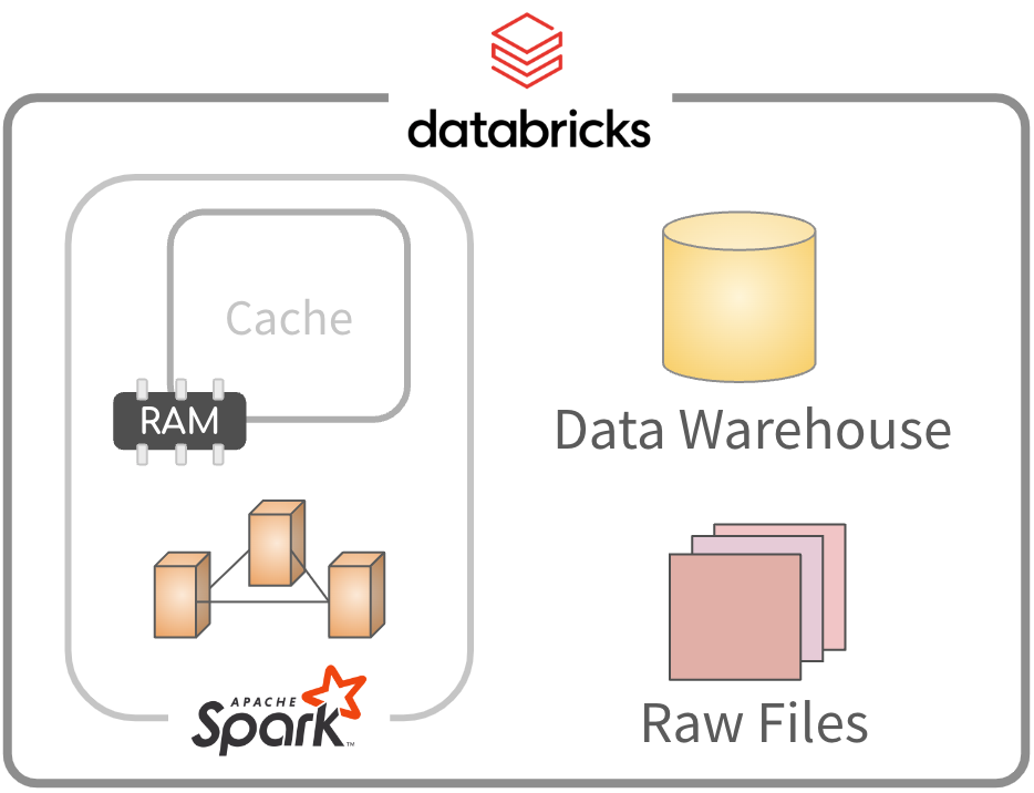
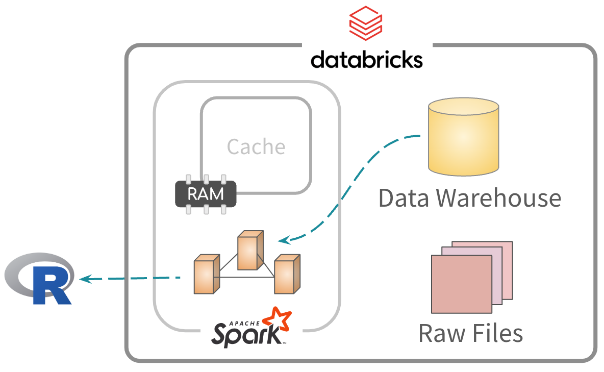
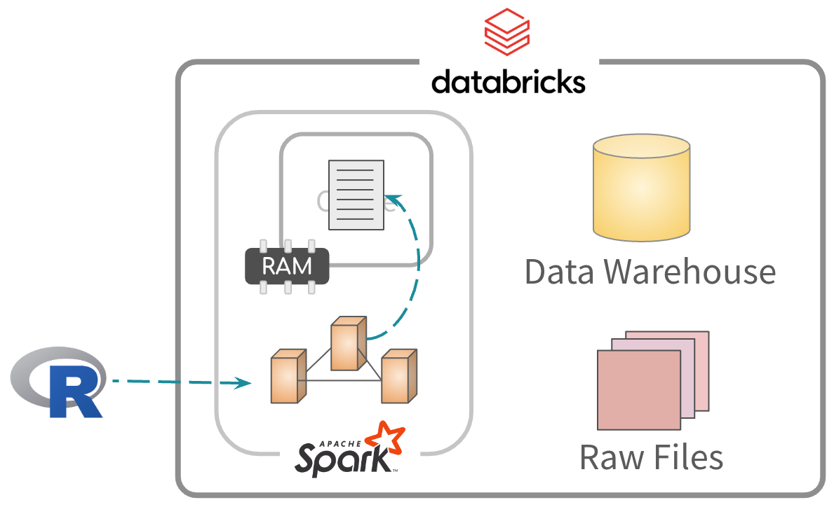
Default approach
Data is read and processed. Results go to R.
Uploading data from R
copy_to() to upload data to Spark
Caching data
2 step process. first, cache all or some data in memory
Caching data
Second, read and process from memory. Much faster

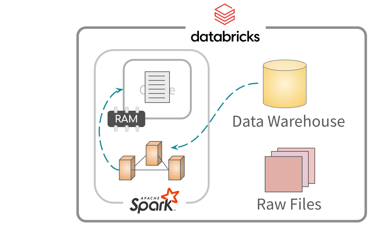
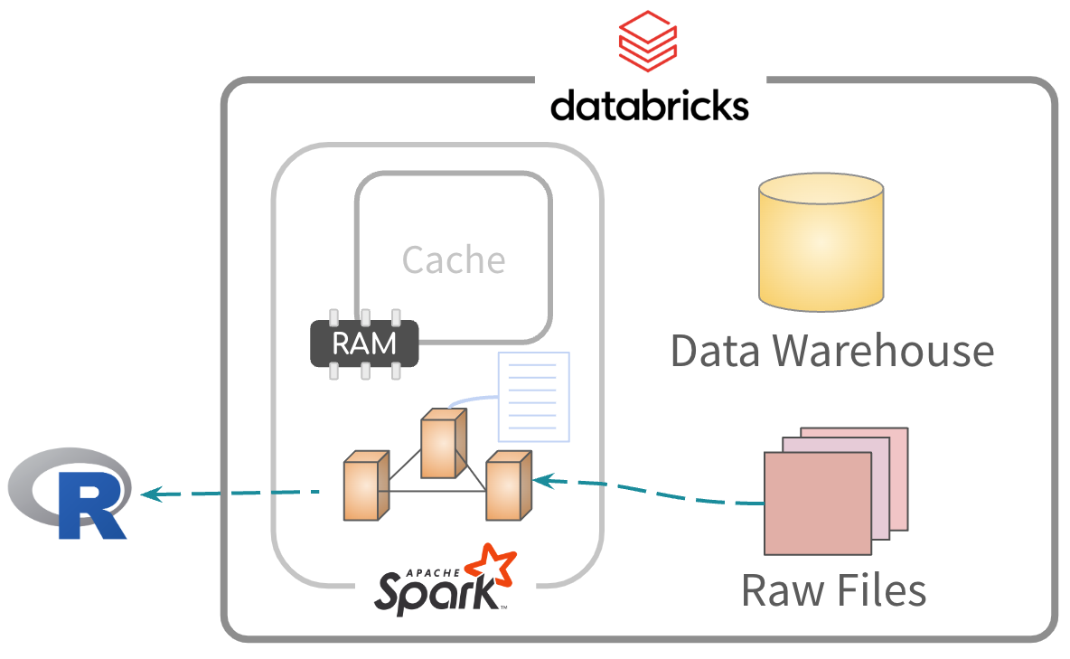
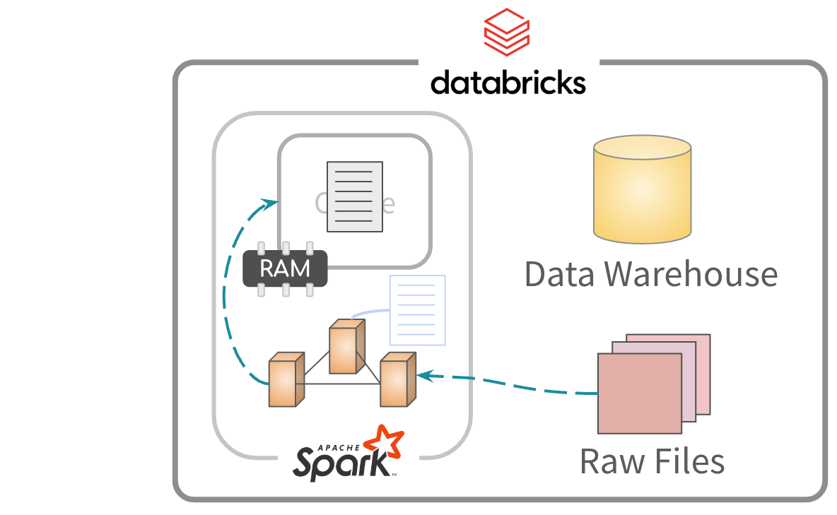
Reading files
By default, files are read and saved to memory
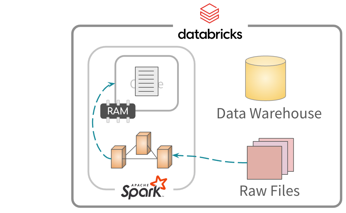
Reading files
Afterwards, the data is read from memory for processing
“Mapping” files
The files can be mapped but not imported to memory
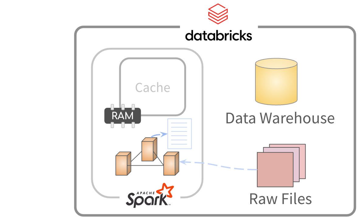
“Mapping” files
Data is read and processed. Results sent to R.
Partial cache
Alternatively, you can cache specific data from the files
Partial cache
Afterwards, the data is read from memory for processing
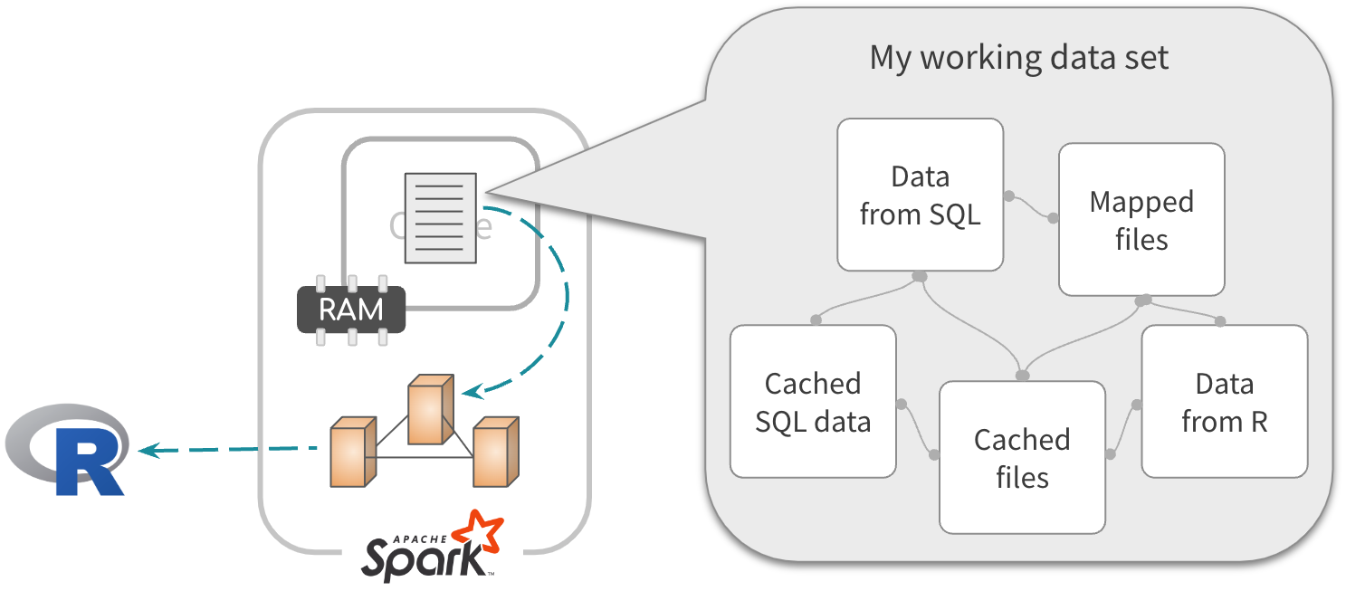
End game
Combine the data from any approach. Cache the resulting table
But first… parallel processing
Spark partitions the data logically
Parallel processing
Each node gets one, or several partitions


Parallel processing
The cluster runs jobs that process each partition in parallel

Parallel processing
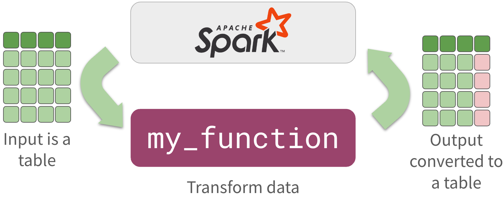
Your R function runs on each partition independently
![]()
![]()
![]()
Parallel processing
Results are appended, and returned to user as a single table
Accessing in R
spark_apply()Enables access to the R run-time installed in the cluster- The R function will run over each individual partition
tbl_mtcars <- copy_to(sc,
                      mtcars)

tbl_mtcars |>
  spark_apply(nrow)
#>       x
#>   <dbl>
#> 1     8
#> 2     8
#> 3     8
#> 4 8Group by variable
Use group_by to override the partitions, and divide data by a column
tbl_mtcars |>
  spark_apply(nrow, group_by = "am")
#> # Source:   table<`sparklyr_tmp_table`> [2 x 2]
#> # Database: spark_connection
#>      am     x
#>   <dbl> <dbl>
#> 1     0    19
#> 2 1 13Custom functions
R function should expect and return a table
R packages
R packages have to be referenced from within your function’s code using library() or ::
tbl_mtcars |>
  spark_apply(function(x) {
      library(broom)
      model <- lm(mpg ~ ., x)
      tidy(model)[1,]
      },
      group_by = "am"
      )
#> # Source:   table<`sparklyr_tmp`> [2 x 6]
#> # Database: spark_connection
#>      am term        estimate std_error statistic p_value
#>   <dbl> <chr>          <dbl>     <dbl>     <dbl>   <dbl>
#> 1     0 (Intercept)     8.64      21.5     0.402   0.697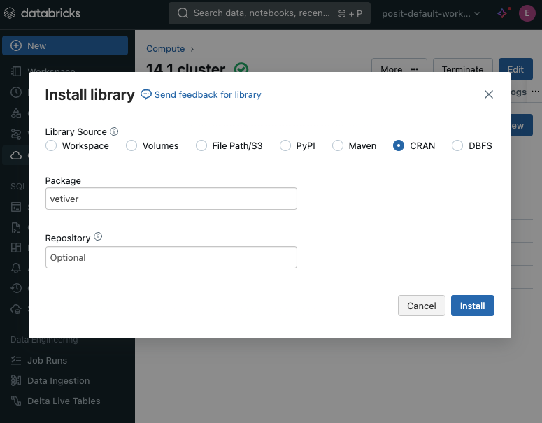
#> 2 1 (Intercept) -138. 69.1 -1.99 0.140Missing packages
- Additional packages can be installed
- In the Databricks portal, use the Libraries tab of the cluster
- Python packages will install from PyPi
- R packages will install from CRAN
In Python
Code sent through gRPC, code runs in remote Python environment through Spark
R UDFs
R code is inserted in a Python script, rpy2 executes
Wrapped Python functions
R:
spark_apply(tbl, my_fun) Python:
tbl.mapInPandas(r_objects.r(my_fun))R:
spark_apply(tbl, my_fun, group_by = "col1") Python:
tbl.applyInPandas.group_by(col1).(r_objects.r(my_fun))Run R models in Spark
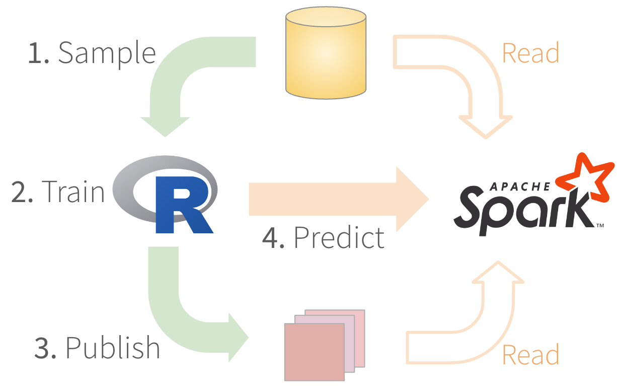
1. Sample - Use dplyr
- Use
dplyr’sslice_sample()function - Download enough data to be representative
local_df <- remote_df |>
 slice_sample(n = 100) |>
collect()2. Train - Ideally, tidymodels
Fit the model locally in R
library(tidymodels)
my_rec <- recipe(x ~ ., data = local_df) |>
  step_normalize(all_numeric_predictors())

my_reg <- linear_reg()

my_wkf <- workflow() |>
  add_model(my_reg) |>
  add_recipe(my_rec)

model <- fit(my_wkf, local_df)3. Publish - Package with vetiver

vetiverpackagestidymodelsworkflows and models- Model is automatically reduced in size
- Output is easy to load into another R session
library(vetiver)
m <- vetiver_model(
 model = model,
 model_name = “model”
 )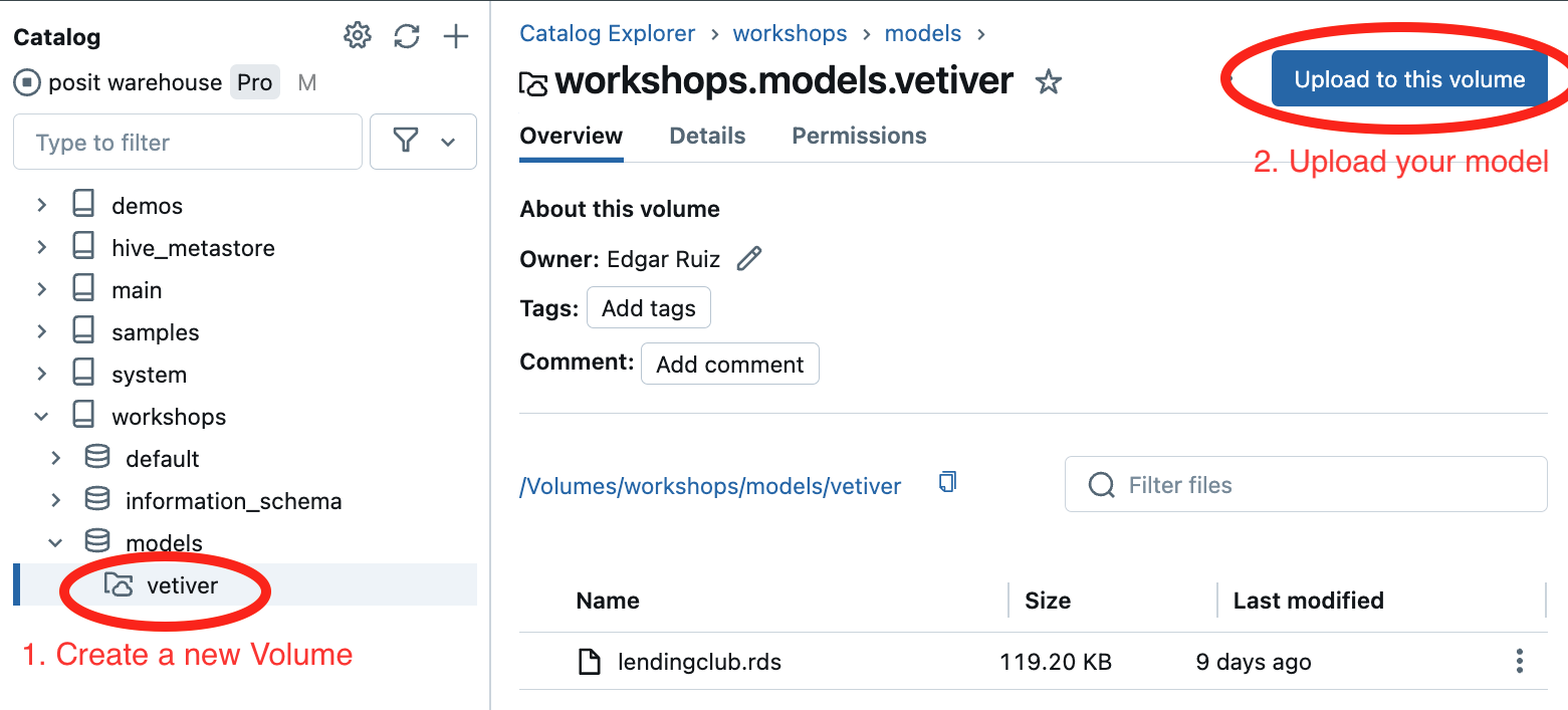
saveRDS(m, “model.rds”)3. Publish - Transfer model file
- Copy the R model where Spark can access
- Location has to be secure
- Options: Databricks UC, s3 buckets, Posit Connect, others
3. Publish - Databricks UC Volume
Run R models in Spark
Call ai functions in dplyr
- Call the
aifunctions viadplyrverbs dbplyrpasses unrecognized functions ‘as-is’ in the query
orders |>
  head() |>
  select(o_comment) |>
  mutate(
    sentiment = ai_analyze_sentiment(o_comment)
    )
#> # Source:   SQL [6 x 2]
#>   o_comment                   sentiment
#>   <chr>                        <chr>
#> 1 ", pending theodolites …    neutral
#> 2 "uriously special foxes …   neutral
#> 3 "sleep. courts after the …  neutral
#> 4 "ess foxes may sleep …      neutral
#> 5 "ts wake blithely unusual … mixed
#> 6 "hins sleep. fluffily … neutralIntroducing chattr

chattris an interface to LLMs (Large Language Models)- It enables interaction with the model directly from RStudio
- Submit a prompt to the LLM from your script, or by using the provided Shiny Gadget.
library(chattr)

chattr("my programming question")

chattr_app()
chattr supports Databricks’ LLM
chattr supports Databricks’ LLM
Big thank you to Zack Davies at Databricks!! 🎉🎉🎉
chattr supports Databricks’ LLM
Automatically makes the options available if it detects your Databricks token.
> chattr_app()
── chattr - Available models
Select the number of the model you would like to use:

1: Databricks - databricks-dbrx-instruct (databricks-dbrx)

2: Databricks - databricks-meta-llama-3-70b-instruct (databricks-meta-llama3-70b)

3: Databricks - databricks-mixtral-8x7b-instruct (databricks-mixtral8x7b)

Selection: 1Important features
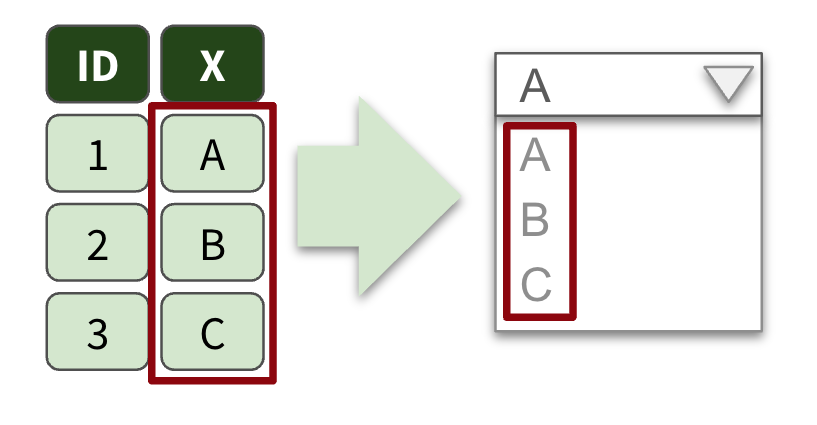
- Data driven dropdowns
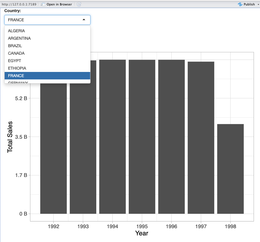
Important features
- Data driven dropdowns
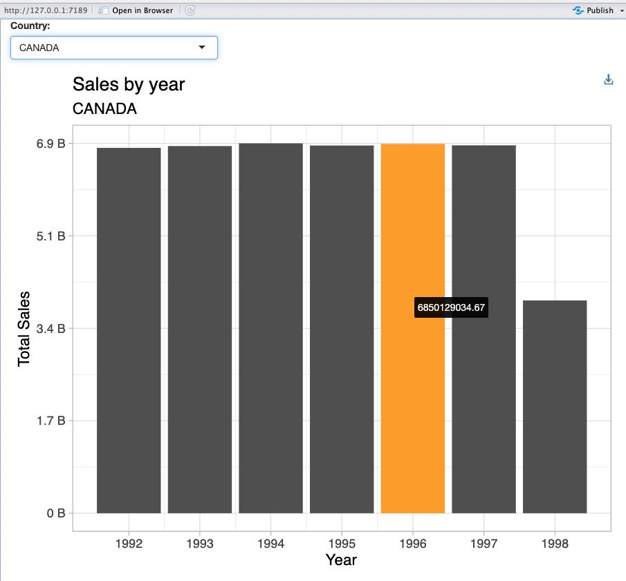
- Interactive plots (hover over)
Important features
- Data driven dropdowns
- Interactive plots (hover over)
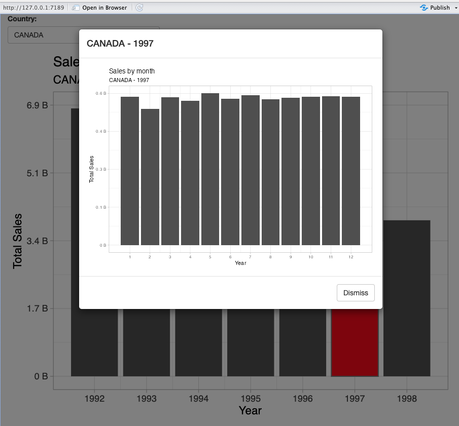
- Drill down when interacting with the plot
Data driven dropdowns
When do we need them?
When options in the data change regularly
Interactive Plots
ggiraph

- Allows you to create dynamic
ggplotgraphs. - Adds tooltips, hover effects, and JavaScript actions
- Enables selecting elements of a plot inside a
shinyapp - Adds interactivity to
ggplotgeometries, legends and theme elements
Plot drill-down
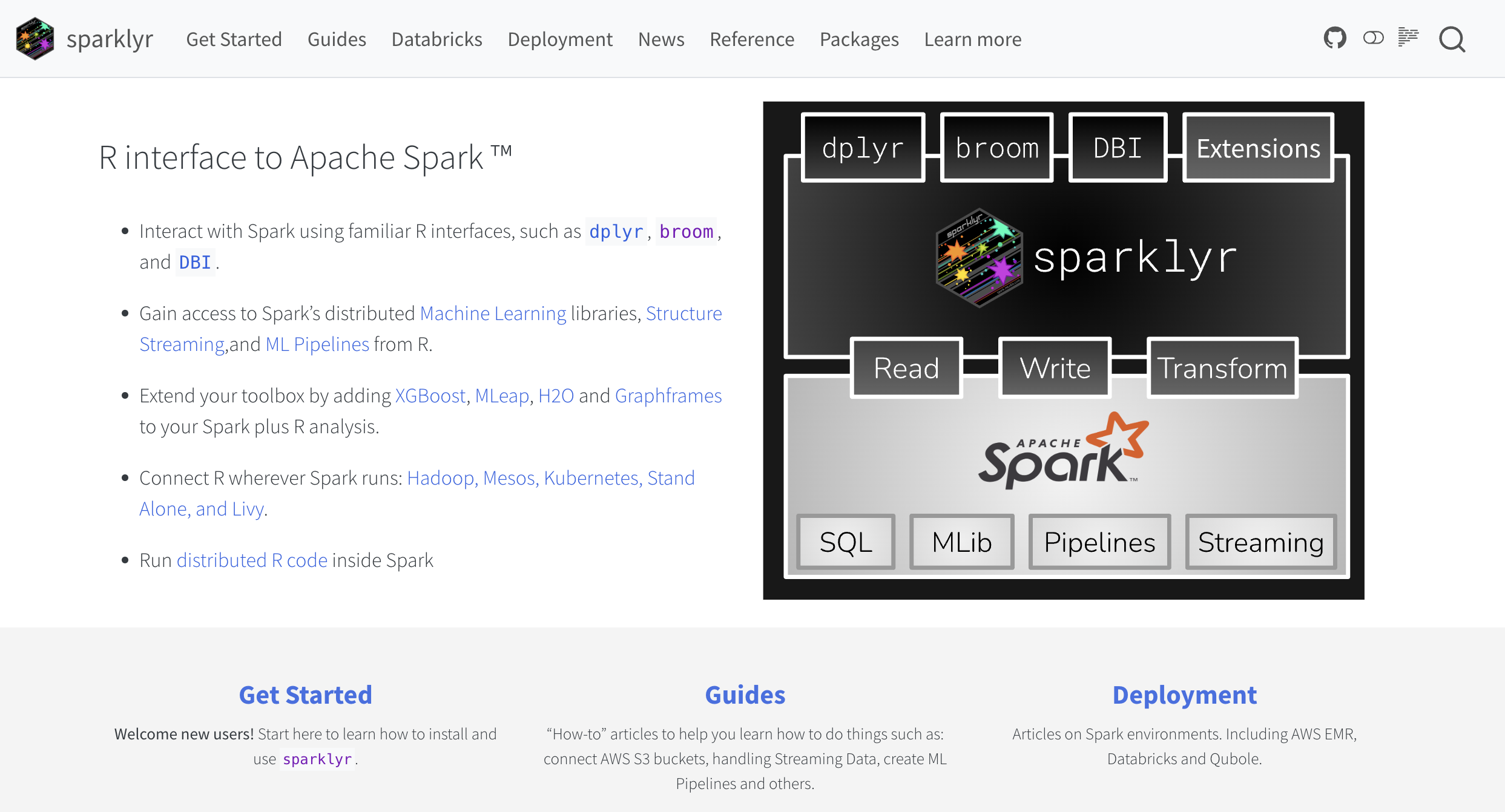
Official Site
spark.posit.co
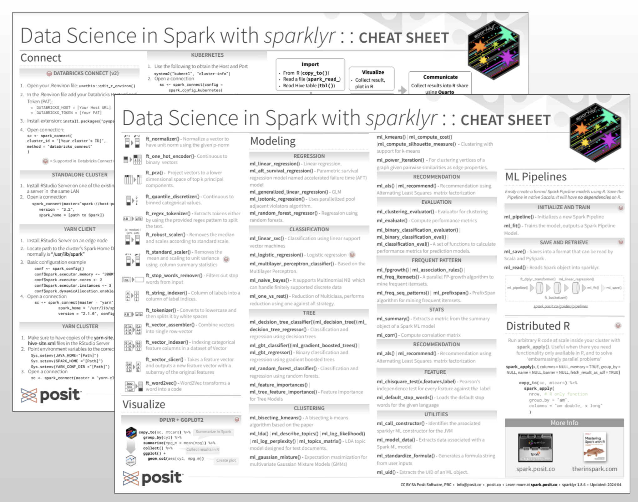
Cheatsheet
spark.posit.co/images/homepage/sparklyr.pdf
Ask questions
forum.posit.co