Modern UI with bslib
Level Up with Shiny for R
posit::conf(2024)
2024-08-12
shiny + bslib = 💛
At first there was shiny

Then came bslib
bslib: 1-line Bootstrap upgrades
bslib: 1-line Bootstrap themes!
bslib: 1-line Bootstrap themes!
bslib: 3-line Bootstrap themes!
bslib: N-line Bootstrap themes!

bslib: A Shiny Bootstrap theme!
bslib: A Shiny Bootstrap preset!
bslib: A Shiny Bootstrap default!
Your Turn
U.S. College Scorecard
We’ll be using the U.S. College Scorecard data for our examples today, from 📦 collegeScorecard.
school- Information about colleges and universities
scorecard- Data on cost, admission and completion rates, earnings and more
Your Turn _exercises/01-app.R
- Run the app and use it to learn about the
schoolandscorecarddatasets. - Load
bsliband change the theme of the app, using your favorite colors for the background and foreground colors.
Hint: Get color inspiration at https://coolors.co. - Choose an accent color for the app’s primary color.
- Add
thematic::thematic_shiny()to the app to make the plots look better.
04:00
bslib: fillable layouts and cards
#| standalone: true
#| components: [editor, viewer]
#| orientation: horizontal
#| viewerHeight: "100%"

# ┌ level-up-shiny ──────────────────────────────────┐
# │                                                  │
# │                    Solution 1                    │
# │                                                  │
# └─────────────────────────────── posit::conf(2024) ┘

library(shiny)
library(bslib)

thematic::thematic_shiny()

ui <- fluidPage(
  theme = bs_theme(
    version = 5,
    bg = "#0B3954",
    fg = "#bfd7ea",
    primary = "#0BAFC1",
  ),
  selectizeInput("data", "Data set", choices = c("school", "scorecard"), selected = "school"),
  radioButtons("type", "Inspection type", choices = c("Column Types" = "types", "Categorical" = "cat", "Numeric" = "num", "Missing" = "na"), inline = TRUE),
  plotOutput("plot")
)

server <- function(input, output, session) {
  data <- reactive({
    switch(
      input$data,
      "school" = collegeScorecard::school,
      "scorecard" = collegeScorecard::scorecard
    )
  })

  output$plot <- renderPlot({
    req(data())

    df <- data()

    inspected <- switch(
      input$type,
      "types" = inspectdf::inspect_types(df),
      "cat" = inspectdf::inspect_cat(df),
      "num" = inspectdf::inspect_num(df),
      "na" = inspectdf::inspect_na(df)
    )

    inspectdf::show_plot(inspected, col_palette = 2)
  })
}

shinyApp(ui, server)


## file: notes.R
# => _exercises/01_solution_app.R

theme = bs_theme(
  version = 5,
  bg = "#0B3954",
  fg = "#bfd7ea",
  primary = "#0BAFC1",
)

# * Add thematic::thematic_shiny() to the app
# * page_fluid()
#| standalone: true
#| components: [editor, viewer]
#| orientation: horizontal
#| viewerHeight: "100%"
library(shiny)
library(bslib)
library(plotly)
library(collegeScorecard)
colors <- c("#007bc2", "#f45100", "#bf007f")
ui <- page_fluid(
plotlyOutput("plot_control")
)
server <- function(input, output, session) {
output$plot_control <- renderPlotly({
plot_school_var(school, "control", title = "School Governance", color = colors[1])
})
output$plot_deg_predominant <- renderPlotly({
plot_school_var(school, "deg_predominant", title = "Predominant Degree", colors[2])
})
output$plot_locale_type <- renderPlotly({
plot_school_var(school, "locale_type", title = "Locale Type", colors[3])
})
}
plot_school_var <- function(school, var, title = "", color = "blue") {
school |>
plot_ly(
y = ~get(var),
type = "histogram",
color = I(color)
) |>
layout(
title = title,
xaxis = list(title = "Number of Schools"),
yaxis = list(title = "")
) |>
config(displayModeBar = FALSE)
}
shinyApp(ui, server)
## file: notes.R
# => examples/02-bslib/01_app.R
# * Compare with page_fillable()
# * fill items and fillable containers
# * Add card()Filling Layouts
Fillable Container 🫱
🫲 Fill Item
Filling Layouts
Fillable Container 🤝 Fill Item
card
plot
Filling Layouts
Fillable Container 🫸 🫲 Fill Item
fillable = FALSE
Filling Layouts
Fillable Container 🫱 🫷 Fill Item
fill = FALSE
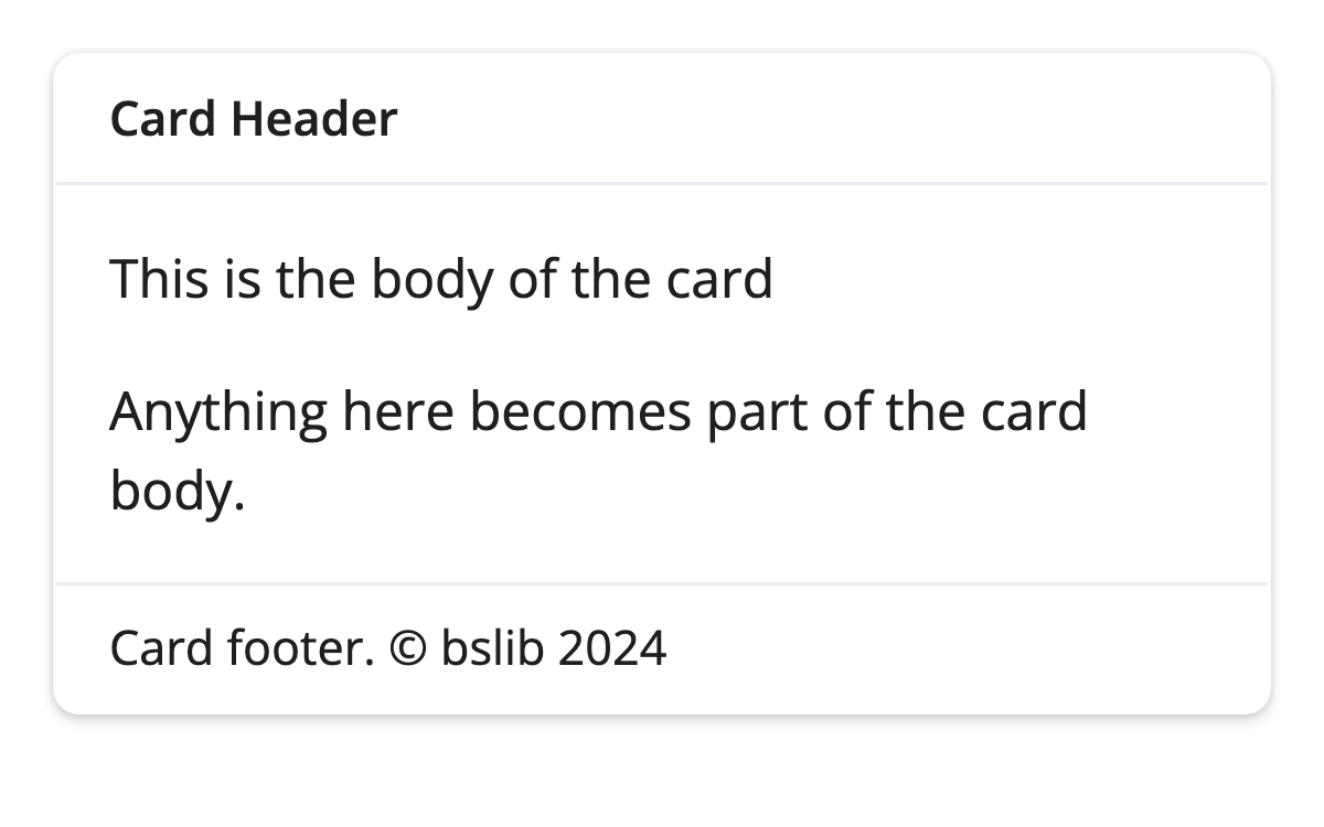
Card Parts
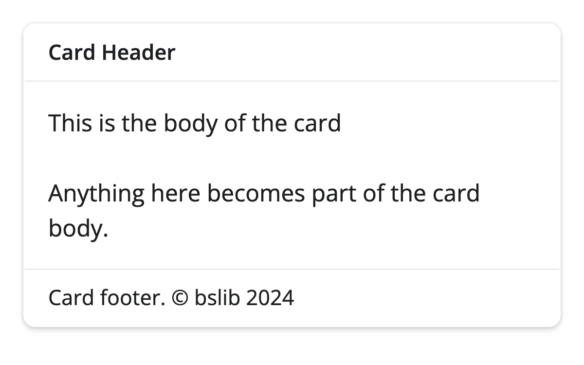
Card Parts
Full Screen Cards
#| standalone: true
#| components: [viewer]
#| viewerHeight: "400px"

library(shiny)
library(bslib)
library(dplyr)
library(ggplot2)
library(collegeScorecard)

# UI -------------------------------------------------------------------------

ui <- page_fillable(
  selectInput("state", "State", choices = setNames(state.abb, state.name)),
  card(
    card_header("Predominant Degree"),
    plotOutput("plot_deg_predominant"),
    full_screen = TRUE
  ),
  card(
    card_header("Cost vs Earnings"),
    plotOutput("plot_cost"),
    full_screen = TRUE
  )
)

# Setup -----------------------------------------------------------------------

colors <- c("#007bc2", "#f45100", "#bf007f")

theme_set(
  theme_minimal(18) +
    theme(
      panel.grid.minor = element_blank(),
      panel.grid.major.y = element_blank(),
      axis.title = element_text(size = 14)
    )
)

scorecard_latest <-
  scorecard |>
  group_by(id) |>
  arrange(academic_year) |>
  tidyr::fill(
    n_undergrads,
    rate_admissions,
    rate_completion,
    cost_avg,
    amnt_earnings_med_10y
  ) |>
  slice_max(academic_year, n = 1, with_ties = FALSE) |>
  ungroup()

school <-
  school |>
  left_join(scorecard_latest, by = "id")

# Server ---------------------------------------------------------------------

server <- function(input, output, session) {
  output$plot_deg_predominant <- renderPlot({
    school |>
      filter(state == input$state) |>
      ggplot() +
      aes(y = deg_predominant) +
      geom_bar(fill = colors[2], na.rm = TRUE) +
      labs(
        title = "Predominant Degree",
        x = "Number of Schools",
        y = NULL
      ) +
      scale_x_continuous(expand = c(0, 0)) +
      scale_y_discrete(
        labels = \(x) ifelse(is.na(x), "Unknown", x)
      )
  })

  output$plot_cost <- renderPlot({
    label_dollars <- scales::label_dollar(scale_cut = scales::cut_long_scale())

    school |>
      filter(state == input$state) |>
      ggplot() +
      aes(
        x = cost_avg,
        y = amnt_earnings_med_10y,
        # color = !!rlang::sym(input$cost_group_by)
      ) +
      geom_point(size = 3, color = colors[1]) +
      labs(
        title = NULL,
        x = "Average Cost",
        y = "Median Earnings",
        color = NULL
      ) +
      scale_x_continuous(labels = label_dollars) +
      scale_y_continuous(labels = label_dollars) +
      # scale_color_manual(
      #   values = c("#007bc2", "#f45100", "#00891a", "#bf007f", "#f9b928", "#03c7e8", "#00bf7f")
      # ) +
      theme(
        legend.position = "bottom",
        panel.grid.major.y = element_line()
      )
  })
}

shinyApp(ui, server)
Your Turn
Your Turn _exercises/02-app.R
- Place each of the plots in a
card()with a header. - What happens when you set
fill = FALSEorfillable = FALSEin a card? - Give each card a minimum height to prevent squishing.
- How is the plotly plot different from the ggplot2 plot?
04:00
Sidebar Layouts
A global page-level sidebar
A global page-level sidebar
Local sidebars
#| standalone: true
#| components: [editor, viewer]
#| orientation: horizontal
#| viewerHeight: "100%"

library(shiny)
library(bslib)
library(dplyr)
library(ggplot2)
library(collegeScorecard)

# UI -------------------------------------------------------------------------

ui <- page_fillable(
  selectInput("state", "State", choices = setNames(state.abb, state.name)),
  card(
    card_header("Predominant Degree"),
    plotOutput("plot_deg_predominant"),
    full_screen = TRUE
  ),
  card(
    card_header("Cost vs Earnings"),
    plotOutput("plot_cost"),
    full_screen = TRUE
  )
)

# Setup -----------------------------------------------------------------------

colors <- c("#007bc2", "#f45100", "#bf007f")

theme_set(
  theme_minimal(18) +
    theme(
      panel.grid.minor = element_blank(),
      panel.grid.major.y = element_blank(),
      axis.title = element_text(size = 14)
    )
)

scorecard_latest <-
  scorecard |>
  group_by(id) |>
  arrange(academic_year) |>
  tidyr::fill(
    n_undergrads,
    rate_admissions,
    rate_completion,
    cost_avg,
    amnt_earnings_med_10y
  ) |>
  slice_max(academic_year, n = 1, with_ties = FALSE) |>
  ungroup()

school <-
  school |>
  left_join(scorecard_latest, by = "id")

# Server ---------------------------------------------------------------------

server <- function(input, output, session) {
  output$plot_deg_predominant <- renderPlot({
    school |>
      filter(state == input$state) |>
      ggplot() +
      aes(y = deg_predominant) +
      geom_bar(fill = colors[2], na.rm = TRUE) +
      labs(
        title = "Predominant Degree",
        x = "Number of Schools",
        y = NULL
      ) +
      scale_x_continuous(expand = c(0, 0)) +
      scale_y_discrete(
        labels = \(x) ifelse(is.na(x), "Unknown", x)
      )
  })

  output$plot_cost <- renderPlot({
    label_dollars <- scales::label_dollar(scale_cut = scales::cut_long_scale())

    school |>
      filter(state == input$state) |>
      ggplot() +
      aes(
        x = cost_avg,
        y = amnt_earnings_med_10y,
        # color = !!rlang::sym(input$cost_group_by)
      ) +
      geom_point(size = 3, color = colors[1]) +
      labs(
        title = NULL,
        x = "Average Cost",
        y = "Median Earnings",
        color = NULL
      ) +
      scale_x_continuous(labels = label_dollars) +
      scale_y_continuous(labels = label_dollars) +
      # scale_color_manual(
      #   values = c("#007bc2", "#f45100", "#00891a", "#bf007f", "#f9b928", "#03c7e8", "#00bf7f")
      # ) +
      theme(
        legend.position = "bottom",
        panel.grid.major.y = element_line()
      )
  })
}

shinyApp(ui, server)


## file: notes.R
# * Use page_sidebar(), move state selector there
# * turn fill on and off for main area
# * Mention `sidebar()` options, like `open` and `position`Your Turn
Your Turn _exercises/03_app.R
04:00
- Convert the app to a page with a sidebar
- One input only applies to one of the plots. Use
layout_sidebar()to create a sidebar with a local input for that plot. - Stretch: Position the local sidebar on the right of the card and have it start closed.
Value Boxes
#| standalone: true
#| components: [editor, viewer]
#| orientation: horizontal
#| viewerHeight: "100%"

library(shiny)
library(bslib)

ui <- page_fluid(
  card(
    "Undergrad Students",
    5612
  ),
  card(
    "Average Yearly Cost",
    32125
  ),
  card(
    "Completion Rate",
    0.83
  )
)

server <- function(input, output, session) {

}

shinyApp(ui, server)


## file: solution.R
library(shiny)
library(bslib)
library(fontawesome)

ui <- page_fluid(
  value_box(
    "Undergrad Students",
    scales::number(5612, big.mark = ","),
    showcase = fa_i("people-roof")
  ),
  value_box(
    "Average Yearly Cost",
    scales::dollar(32125),
    showcase = fa_i("money-check-dollar"),
    theme = "primary"
  ),
  value_box(
    "Completion Rate",
    scales::percent(0.83),
    showcase = fa_i("user-graduate"),
    theme = "bg-gradient-orange-red"
  )
)

server <- function(input, output, session) {

}

shinyApp(ui, server)Build-A-Box
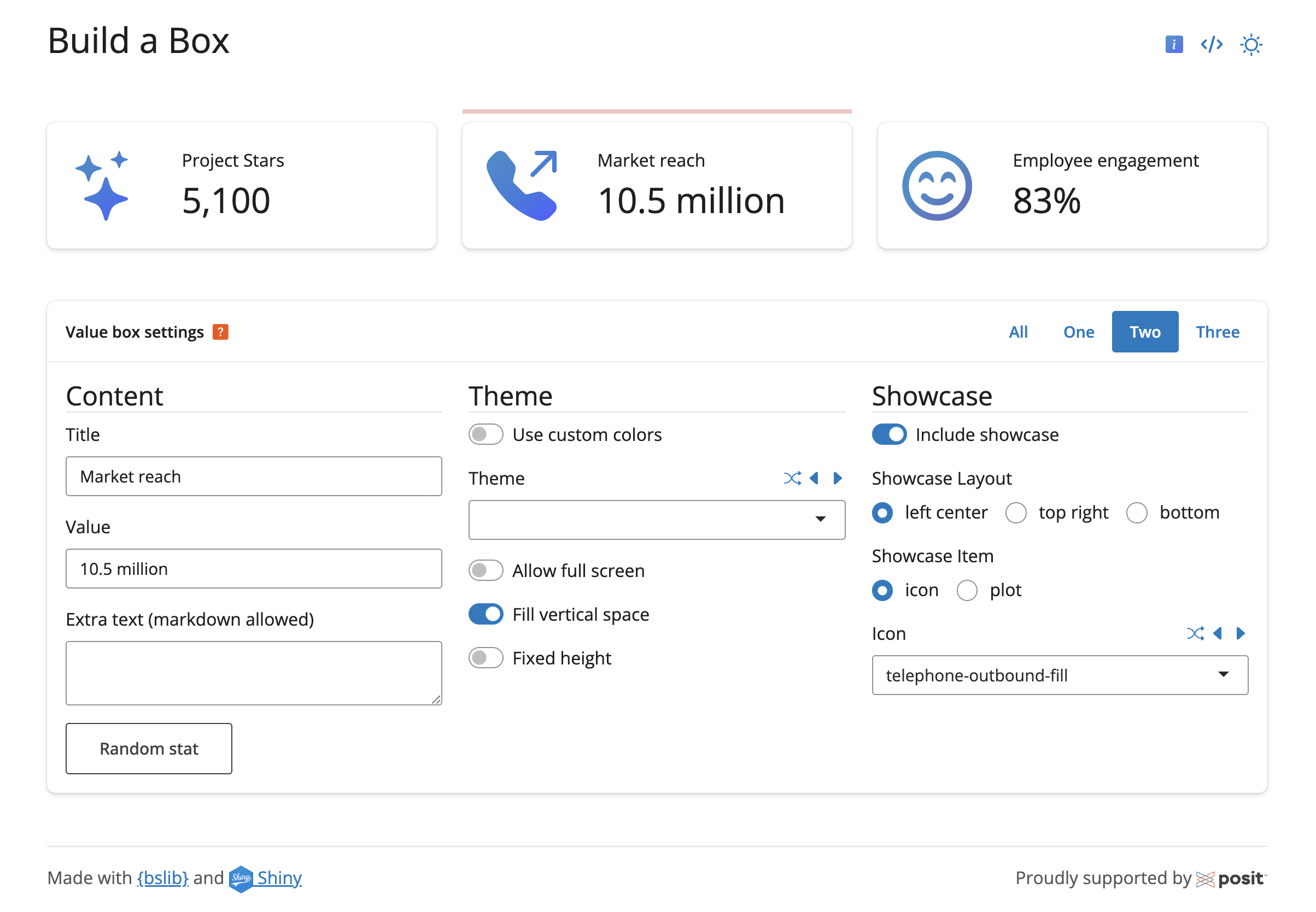
Your Turn
Your Turn _exercises/04_app.R
06:00
- Use the Build-A-Box app to design three value boxes
- bslib.shinyapps.io/build-a-box
shiny::runExample("build-a-box", package = "bslib")
- Some icon hints:
- public -
fa_i("university") - non-profit -
fa_i("school-lock")(it’s still private!) - for-profit -
fa_i("building")
- public -
Column Layouts
Column Layouts
layout_column_wrap()
layout_columns()
Takes any number of items and lays them out column-wise
Takes any number of items and lays them out column-wise
Equally sized columns and rows
Uneven columns and rows
Best when all items are the same thing
Best for using Bootstrap’s 12-column grid
Splat!
#| standalone: true
#| components: [editor, viewer]
#| orientation: horizontal
#| viewerHeight: "100%"

library(shiny)
library(bslib)
library(glue)
library(dplyr)
library(purrr)
library(collegeScorecard)

ui <- page_fluid(
  class = "p-4",
  sliderInput("n", "Top N Schools", min = 1, max = 20, value = 9, ticks = FALSE),
  uiOutput("layout_school_cards")
)

server <- function(input, output, session) {
  colors <- c("blue", "indigo", "purple", "pink", "red", "orange", "yellow", "green", "teal", "cyan")

  output$layout_school_cards <- renderUI({
    school_cards()
  })

  school_cards <- reactive({
    set.seed(42**3.8)

    pmap(top_n_schools(), function(name, cost_avg, city, state, ...) {
      # Turn this into a value box
      p(
        strong(name),
        glue("{city}, {state}")
      )
    })
  })

  top_n_schools <- reactive({
    scorecard |>
      filter(n_undergrads > 1000) |>
      slice_max(academic_year, n = 1) |>
      slice_max(cost_avg, n = input$n) |>
      arrange(desc(cost_avg)) |>
      left_join(school, by = "id")
  })
}

shinyApp(ui, server)


## file: notes.R
value_box(
  title = name,
  value = scales::dollar(cost_avg),
  theme = sample(colors, 1),
  p(glue("{city}, {state}"))
)

# * write out `value_box()` code
# * `layout_columns()` vs `layout_column_wrap()`
# * `width` vs `col_widths`
Your Turn
Your Turn _exercises/05_app.R
04:00
Use
layout_columns()andlayout_column_wrap()to improve the layout of the app.Some hints:
- Which items should be grouped together in a row?
layout_columns()hascol_widthswhich takes a vector of column widths in Bootstrap’s grid units.layout_column_wrap()haswidthand can take fractional widths, e.g.1 / 2.
Details on Demand
#| standalone: true
#| components: [editor, viewer]
#| orientation: horizontal
#| viewerHeight: "100%"

library(shiny)
library(bslib)
library(fontawesome)
library(collegeScorecard)

ui <- page_fillable(
  selectInput("state", "State", choices = setNames(state.abb, state.name)),
  checkboxGroupInput("locale_type", "Locale Type", choices = levels(school$locale_type), selected = levels(school$locale_type)),
  sliderInput("n_undergrads", "Number of Undergrads", min = 0, max = 50000, value = c(0, 50000), step = 1000)
)

server <- function(input, output, session) {

}

shinyApp(ui, server)


## file: notes.R
# * accordion()
# * accordion_panel()
# * fa_i: map, users

## file: solution.R
library(shiny)
library(bslib)
library(fontawesome)
library(collegeScorecard)

ui <- page_fillable(
  accordion(
    multiple = FALSE,
    accordion_panel(
      title = "Location",
      icon = fa_i("map"),
      selectInput("state", "State", choices = setNames(state.abb, state.name)),
      checkboxGroupInput("locale_type", "Locale Type", choices = levels(school$locale_type), selected = levels(school$locale_type)),
    ),
    accordion_panel(
      title = "Student Population",
      icon = fa_i("users"),
      sliderInput("n_undergrads", "Number of Undergrads", min = 0, max = 50000, value = c(0, 50000), step = 1000),
    )
  )
)

server <- function(input, output, session) {

}

shinyApp(ui, server)
#| standalone: true
#| components: [editor, viewer]
#| orientation: horizontal
#| viewerHeight: "100%"
library(shiny)
library(bslib)
library(fontawesome)
ui <- page_fillable(
class = "justify-content-center align-items-center",
)
server <- function(input, output, session) {
}
shinyApp(ui, server)
## file: notes.R
tooltip(
fontawesome::fa_i("info-circle"),
"Hover over me for more info!"
)
textInput("package", "Package Name", placeholder = "e.g. shiny")#| standalone: true
#| components: [editor, viewer]
#| orientation: horizontal
#| viewerHeight: "100%"
library(shiny)
library(bslib)
library(fontawesome)
ui <- page_fillable(
class = "justify-content-center align-items-center",
)
server <- function(input, output, session) {
}
shinyApp(ui, server)
## file: notes.R
# * The target can be anything, typically a `button()` or icon
# * `{bsicons}` or `{fontawesome}`
# * Important to give the icon a title
#
# * The content can be anything, including inputs!
popover(
fontawesome::fa_i("gear", title = "Settings"),
title = "Plot settings",
"I'm the popover content."
)
card(
card_header("Card Title"),
"A map or a plot would go here.",
max_height = 300
)
card(
card_header(
class = "hstack",
"Card Title",
popover(
fontawesome::fa_i("gear", title = "Settings", class = "ms-auto"),
title = "Plot settings",
checkboxInput("show_legend", "Show legend", TRUE),
input_switch("show_legend", "Show legend", TRUE)
)
),
"A map or a plot would go here.",
max_height = 300
)Popover in a card header
card(
  card_header(
    class = "hstack",
    "Card Title",
    popover(
      fontawesome::fa_i("gear", title = "Settings", class = "ms-auto"),
      title = "Plot settings",
      input_switch("show_legend", "Show legend", TRUE)
    )
  ),
  "A map or a plot would go here."
)
https://getbootstrap.com/docs/5.3/helpers/stacks/#horizontal
Your Turn
Your Turn _exercises/06_app.R
08:00
- Use
accordion()andaccordion_panel()to organize the sidebar inputs. See the exercise header for links to search icons. - Add informational tooltips to the value box titles.
- Public: “Supported by public funds and operated by elected or appointed officials.”
- Nonprofit: “Private institutions that are not operated for profit.”
- For-Profit: “Operated by private, profit-seeking businesses.”
- Stretch: Replace the local sidebar with a popover element.