Fast Apps 🏎️💨

Level Up with Shiny for R

posit::conf(2024)

2024-08-12

Is this app fast?

shiny::runApp("_examples/09-fast-apps/01_app.R")

Is this app fast?

shiny::runApp("_examples/09-fast-apps/02_app.R")

How long does this take?

Done!

Your Turn

Your Turn `_exercises/10_app.R`

04:00

Add useBusyIndicators() to the UI (anywhere you want, really).
Use busyIndicatorOptions() to pick a different spinner type or color.
Stretch: Use the spinner_selector argument to pick a different spinner type for each card. (Hint: each card has a unique class.)

Caching

It’s still slow, but at least it’s only slow once!

bindCache()

output$slow_plot <- renderPlot({
  data() |>
    why_does_this_take_so_long(input$plot_type)
})

bindCache()

output$slow_plot <- renderPlot({
  data() |>
    why_does_this_take_so_long(input$plot_type)
}) |>
  bindCache(data(), input$plot_type)

bindCache()

output$slow_plot <- renderPlot({
  data() |>
    why_does_this_take_so_long(input$plot_type)
}) |>
  bindCache(data(), input$plot_type)

slow_data <- reactive({
  fetch_from_slow_api(input$data_type)
})

bindCache()

output$slow_plot <- renderPlot({
  data() |>
    why_does_this_take_so_long(input$plot_type)
}) |>
  bindCache(data(), input$plot_type)

slow_data <- reactive({
  fetch_from_slow_api(input$data_type)
}) |>
  bindCache(input$data_type)

More about caching

Shiny - Using caching in Shiny to maximize performance

Your Turn

Your Turn `_exercises/11_app.R`

04:00

Use bindCache() in your server logic to speed up the app.
Stretch: Is it better to cache the data or the plots? Why?

Make it faster

Why is it slow?

Enter `profvis`

profvis::profvis(
  shiny::runApp("_exercises/10_solution_app.R")
)

Benchmark your options

first_try <- function(n) {
  x <- c()
  for (i in seq_len(n)) {
    x <- c(x, i + runif(1))
  }
  x
}

second_try <- function(n) {
  x <- numeric(n)
  for (i in seq_len(n)) {
    x[i] <- i + runif(1)
  }
  x
}

Benchmark your options

bench::mark(
  first_try(1e4),
  second_try(1e4)
)

Error: Each result must equal the first result:
`first_try(10000)` does not equal `second_try(10000)`

Benchmark your options

bench::mark(
  first_try(1e4),
  second_try(1e4),
  check = FALSE
)

# A tibble: 2 × 6
  expression             min   median `itr/sec` mem_alloc `gc/sec`
  <bch:expr>        <bch:tm> <bch:tm>     <dbl> <bch:byt>    <dbl>
1 first_try(10000)  128.02ms  132.4ms      7.58     382MB     66.4
2 second_try(10000)   4.05ms   4.24ms    224.      78.2KB     18.0

third_try <- function(n) {
  seq_len(n) + runif(n)
}

Benchmark your options

bench::mark(
  first_try(1e4),
  second_try(1e4),
  third_try(1e4),
  check = FALSE
)

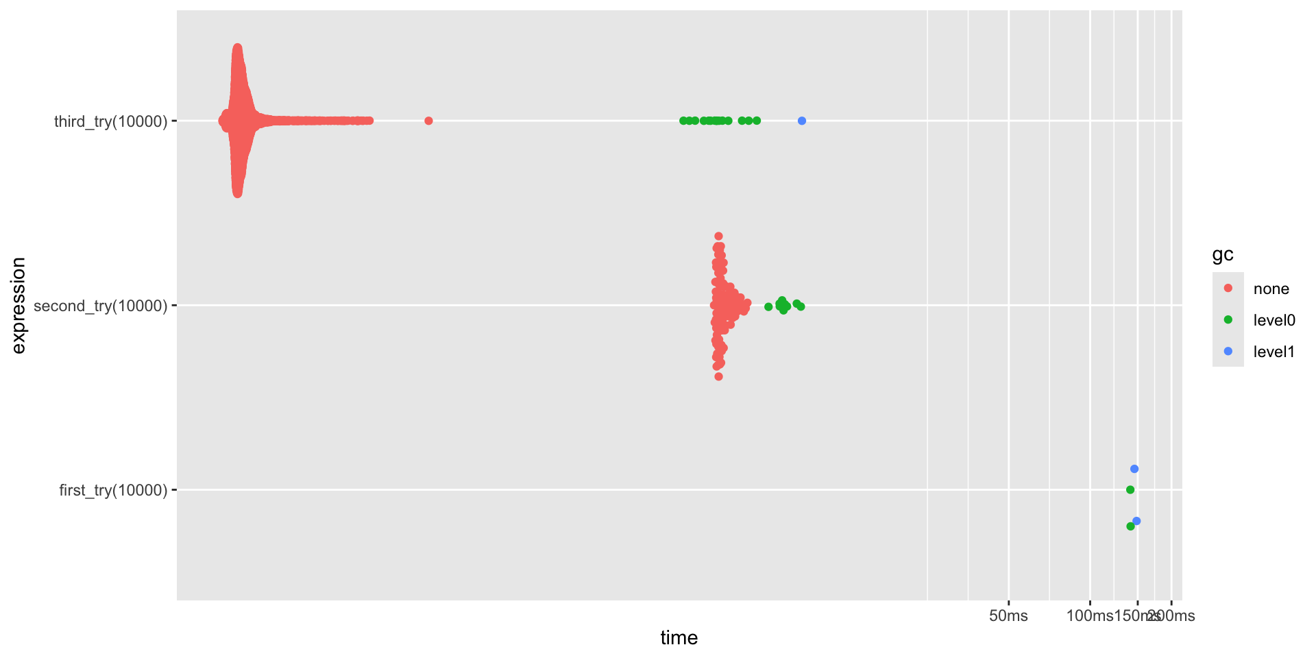
# A tibble: 3 × 6
  expression             min   median `itr/sec` mem_alloc `gc/sec`
  <bch:expr>        <bch:tm> <bch:tm>     <dbl> <bch:byt>    <dbl>
1 first_try(10000)     130ms 135.36ms      7.35     382MB     71.7
2 second_try(10000)   4.08ms   4.28ms    221.      78.2KB     19.9
3 third_try(10000)   61.46µs   70.4µs  10511.     117.3KB     30.0

Benchmark your options

res <- bench::mark(
  first_try(1e4), second_try(1e4), third_try(1e4),
  check = FALSE
)
plot(res)

Your Turn

Your Turn `_exercises/12_slow_app/app.R`

08:00

Use profvis find the slow calls in the app.
Use reactlog to figure out how the structure of the app makes the slow calls worse.
Use bench to compare the performance of two API-calling functions: get_schools_in_state_with_sat() and get_schools_in_state().
How fast can you make the app? Think through or outline your strategy.
Stretch: Implement your strategy and see how much you can improve the app’s performance.

Slow Data, Fast Data

Where does this show up in the reactive graph?

library(shiny)
library(bslib)

ui <- page_fluid(
  # ui stuff...
)

server <- function(input, output, session) {
  scorecard <- read_csv("scorecard.csv")

  # server stuff...
}

shinyApp(ui, server)

Where does this show up in the reactive graph?

library(shiny)
library(bslib)

scorecard <- read_csv("scorecard.csv")

ui <- page_fluid(
  # ui stuff...
)

server <- function(input, output, session) {
  # server stuff...
}

shinyApp(ui, server)

How & where you load data matters

# A tibble: 2 × 2
  path                 size
  <chr>         <fs::bytes>
1 scorecard.csv        338M
2 scorecard.rds        668M

bench::mark(
  readr::read_csv(scorecard_csv),
  readr::read_rds(scorecard_rds),
  check = FALSE
)

# A tibble: 2 × 6
  expression                          min   median `itr/sec` mem_alloc `gc/sec`
  <bch:expr>                     <bch:tm> <bch:tm>     <dbl> <bch:byt>    <dbl>
1 readr::read_csv(scorecard_csv)    1.55s    1.55s     0.647     674MB    0.647
2 readr::read_rds(scorecard_rds) 942.47ms 942.47ms     1.06      643MB    0

It’s a duckdb world now

library(duckdb)

con <- DBI::dbConnect(duckdb(), ":memory:")

scorecard <- duckdb::tbl_file(con, scorecard_csv)

scorecard

# Source:   SQL [?? x 24]
# Database: DuckDB v1.0.0 [root@Darwin 23.5.0:R 4.4.1/:memory:]
       id academic_year n_undergrads cost_tuition_in cost_tuition_out cost_books
    <dbl> <chr>         <chr>        <chr>           <chr>            <chr>     
 1 100654 1996-97       3852         NA              NA               NA        
 2 100663 1996-97       9889         NA              NA               NA        
 3 100672 1996-97       295          NA              NA               NA        
 4 100690 1996-97       60           NA              NA               NA        
 5 100706 1996-97       3854         NA              NA               NA        
 6 100724 1996-97       4679         NA              NA               NA        
 7 100751 1996-97       13948        NA              NA               NA        
 8 100760 1996-97       1792         NA              NA               NA        
 9 100812 1996-97       2698         NA              NA               NA        
10 100830 1996-97       4541         NA              NA               NA        
# ℹ more rows
# ℹ 18 more variables: cost_room_board_on <chr>, cost_room_board_off <chr>,
#   cost_avg <chr>, cost_avg_income_0_30k <chr>, cost_avg_income_30_48k <chr>,
#   cost_avg_income_48_75k <chr>, cost_avg_income_75_110k <chr>,
#   cost_avg_income_110k_plus <chr>, amnt_earnings_med_10y <chr>,
#   rate_completion <chr>, rate_admissions <chr>, score_sat_avg <chr>,
#   score_act_p25 <chr>, score_act_p75 <chr>, score_sat_verbal_p25 <chr>, …

scorecard |>
  filter(academic_year == "2022-23")

# Source:   SQL [?? x 24]
# Database: DuckDB v1.0.0 [root@Darwin 23.5.0:R 4.4.1/:memory:]
       id academic_year n_undergrads cost_tuition_in cost_tuition_out cost_books
    <dbl> <chr>         <chr>        <chr>           <chr>            <chr>     
 1 100654 2022-23       5196         10024           18634            1600      
 2 100663 2022-23       12776        8832            21216            1200      
 3 100690 2022-23       228          NA              NA               NA        
 4 100706 2022-23       6985         11878           24770            2416      
 5 100724 2022-23       3296         11068           19396            1600      
 6 100751 2022-23       31360        11940           32300            800       
 7 100760 2022-23       963          4990            8740             1250      
 8 100812 2022-23       2465         NA              NA               NA        
 9 100830 2022-23       3307         9100            19348            1200      
10 100858 2022-23       25234        12176           32960            1200      
# ℹ more rows
# ℹ 18 more variables: cost_room_board_on <chr>, cost_room_board_off <chr>,
#   cost_avg <chr>, cost_avg_income_0_30k <chr>, cost_avg_income_30_48k <chr>,
#   cost_avg_income_48_75k <chr>, cost_avg_income_75_110k <chr>,
#   cost_avg_income_110k_plus <chr>, amnt_earnings_med_10y <chr>,
#   rate_completion <chr>, rate_admissions <chr>, score_sat_avg <chr>,
#   score_act_p25 <chr>, score_act_p75 <chr>, score_sat_verbal_p25 <chr>, …

scorecard |>
  count()

# Source:   SQL [1 x 1]
# Database: DuckDB v1.0.0 [root@Darwin 23.5.0:R 4.4.1/:memory:]
        n
    <dbl>
1 3666120

It’s a duckdb world now

# A tibble: 3 × 6
  expression                           min   median `itr/sec` mem_alloc `gc/sec`
  <bch:expr>                      <bch:tm> <bch:tm>     <dbl> <bch:byt>    <dbl>
1 readr::read_csv(scorecard_csv)     1.52s    1.52s     0.656     672MB    0.656
2 readr::read_rds(scorecard_rds)  885.77ms 885.77ms     1.13      643MB    1.13 
3 duckdb::tbl_file(con, scorecar…  50.77ms  51.91ms    19.3        52KB    0

duckdb and parquet is an unbeatable combo

# A tibble: 2 × 6
  expression          min   median `itr/sec` mem_alloc `gc/sec`
  <bch:expr>     <bch:tm> <bch:tm>     <dbl> <bch:byt>    <dbl>
1 duckdb_csv      51.12ms  51.86ms      19.2      52KB     0   
2 duckdb_parquet   4.95ms   5.82ms     168.     59.1KB     8.60

.csv file ~ 330 MB
.rds file ~ 670 MB
.parquet file ~ 120 MB

scorecard <- tbl(con, "read_parquet('scorecard.parquet')")

Fast Apps 🏎️💨

Is this app fast?

Is this app fast?

How long does this take?

Your Turn

Your Turn _exercises/10_app.R

Caching

bindCache()

bindCache()

bindCache()

bindCache()

Your Turn

Your Turn _exercises/11_app.R

Make it faster

Why is it slow?

Enter profvis

Benchmark your options

Benchmark your options

Benchmark your options

Benchmark your options

Benchmark your options

Your Turn

Your Turn _exercises/12_slow_app/app.R

Slow Data, Fast Data

Where does this show up in the reactive graph?

Where does this show up in the reactive graph?

How & where you load data matters

It’s a duckdb world now

It’s a duckdb world now

duckdb and parquet is an unbeatable combo

Your Turn `_exercises/10_app.R`

Your Turn `_exercises/11_app.R`

Enter `profvis`

Your Turn `_exercises/12_slow_app/app.R`