Classification II: evaluation & tuning

Session learning objectives

By the end of the session, learners will be able to do the following:

Describe what training, validation, and test data sets are and how they are used in classification.
Split data into training, validation, and test data sets.
Describe what a random seed is and its importance in reproducible data analysis.
Set the random seed in Python using the numpy.random.seed function.
Describe and interpret accuracy, precision, recall, and confusion matrices.

Session learning objectives cont’d

By the end of the session, learners will be able to do the following:

Evaluate classification accuracy, precision, and recall in Python using a test set, a single validation set, and cross-validation.
Produce a confusion matrix in Python.
Choose the number of neighbors in a K-nearest neighbors classifier by maximizing estimated cross-validation accuracy.
Describe underfitting and overfitting, and relate it to the number of neighbors in K-nearest neighbors classification.
Describe the advantages and disadvantages of the K-nearest neighbors classification algorithm.

Evaluating performance

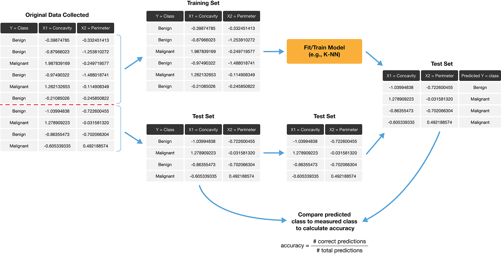
Sometimes our classifier might make the wrong prediction.
A classifier does not need to be right 100% of the time to be useful, though we don’t want the classifier to make too many wrong predictions.
How do we measure how “good” our classifier is?

Data splitting

The trick is to split the data into a training set and test set.
Only the training set when building the classifier.
To evaluate the performance of the classifier, we first set aside the labels from the test set, and then use the classifier to predict the labels in the test set.
If our predictions match the actual labels for the observations in the test set, then we have some confidence that our classifier might also accurately predict the class labels for new observations without known class labels.

Splitting the data into training and testing sets

Prediction accuracy

\[\mathrm{accuracy} = \frac{\mathrm{number \; of \; correct \; predictions}}{\mathrm{total \; number \; of \; predictions}}\]

Is knowing accuracy enough?

Example accuracy calculation:

\[\mathrm{accuracy} = \frac{\mathrm{number \; of \; correct \; predictions}}{\mathrm{total \; number \; of \; predictions}} = \frac{58}{65} = 0.892\]

Prediction accuracy only tells us how often the classifier makes mistakes in general, but does not tell us anything about the kinds of mistakes the classifier makes.
The confusion matrix tells a more complete story.

Example confusion matrix for the breast cancer data:

	Predicted Malignant	Predicted Benign
Actually Malignant	1	3
Actually Benign	4	57

True Positive: A malignant observation that was classified as malignant (top left).
False Positive: A benign observation that was classified as malignant (bottom left).
True Negative: A benign observation that was classified as benign (bottom right).
False Negative: A malignant observation that was classified as benign (top right).

Precision & recall

Precision quantifies how many of the positive predictions the classifier made were actually positive.

\[\mathrm{precision} = \frac{\mathrm{number \; of \; correct \; positive \; predictions}}{\mathrm{total \; number \; of \; positive \; predictions}}\]

Recall quantifies how many of the positive observations in the test set were identified as positive.

\[\mathrm{recall} = \frac{\mathrm{number \; of \; correct \; positive \; predictions}}{\mathrm{total \; number \; of \; positive \; test \; set \; observations}}\]

Precision and recall for the breast cancer data set example

	Predicted Malignant	Predicted Benign
Actually Malignant	1	3
Actually Benign	4	57

\[\mathrm{precision} = \frac{1}{1+4} = 0.20, \quad \mathrm{recall} = \frac{1}{1+3} = 0.25\]

So even with an accuracy of 89%, the precision and recall of the classifier were both relatively low. For this data analysis context, recall is particularly important: if someone has a malignant tumor, we certainly want to identify it. A recall of just 25% would likely be unacceptable!

Randomness and seeds

Our data analyses will often involve the use of randomness
We use randomness any time we need to make a decision in our analysis that needs to be fair, unbiased, and not influenced by human input (e.g., splitting into training and test sets).
However, the use of randomness runs counter to one of the main tenets of good data analysis practice: reproducibility…
The trick is that in Python—and other programming languages—randomness is not actually random! Instead, Python uses a random number generator that produces a sequence of numbers that are completely determined by a seed value.
Once you set the seed value, everything after that point may look random, but is actually totally reproducible.

Setting the seed in Python

Let’s say we want to make a series object containing the integers from 0 to 9. And then we want to randomly pick 10 numbers from that list, but we want it to be reproducible.

import numpy as np
import pandas as pd

np.random.seed(1)

nums_0_to_9 = pd.Series([0, 1, 2, 3, 4, 5, 6, 7, 8, 9])

random_numbers1 = nums_0_to_9.sample(n=10).to_list()
random_numbers1

[2, 9, 6, 4, 0, 3, 1, 7, 8, 5]

You can see that random_numbers1 is a list of 10 numbers from 0 to 9 that, from all appearances, looks random. If we run the sample method again, we will get a fresh batch of 10 numbers that also look random.

random_numbers2 = nums_0_to_9.sample(n=10).to_list()
random_numbers2

[9, 5, 3, 0, 8, 4, 2, 1, 6, 7]

Setting the seed in Python (cont’d)

If we choose a different value for the seed—say, 4235—we obtain a different sequence of random numbers:

# seed was 1 on the last slide when we generated this list
random_numbers1

[2, 9, 6, 4, 0, 3, 1, 7, 8, 5]

np.random.seed(4235)
random_numbers1_different = nums_0_to_9.sample(n=10).to_list()

random_numbers1
random_numbers1_different

[6, 7, 2, 3, 5, 9, 1, 4, 0, 8]

Back to the breast cancer data set example

# load packages
import altair as alt
import pandas as pd
from sklearn import set_config

# Output dataframes instead of arrays
set_config(transform_output="pandas")

# set the seed
np.random.seed(3)

# load data
cancer = pd.read_csv("data/wdbc_unscaled.csv")
# re-label Class "M" as "Malignant", and Class "B" as "Benign"
cancer["Class"] = cancer["Class"].replace({
    "M" : "Malignant",
    "B" : "Benign"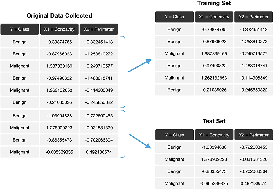
})

Breast cancer data

perim_concav = alt.Chart(cancer).mark_circle().encode(
    x=alt.X("Smoothness").scale(zero=False),
    y="Concavity",
    color=alt.Color("Class").title("Diagnosis")
)

Create the train / test split

Before fitting any models, or doing exploratory data analysis, it is critical that you split the data into training and test sets.
Typically, the training set is between 50% and 95% of the data, while the test set is the remaining 5% to 50%.
The train_test_split function from scikit-learn handles the procedure of splitting the data for us.
Use shuffle=True to remove the influence of order in the data set.
Set the stratify parameter to be the response variable to ensure the same proportion of each class ends up in both the training and testing sets.

Splitting the breast cancer data set

Split the data so 75% are in the training set, and 25% in the test set
Data are shuffled
Split is stratified on the Class variable

from sklearn.model_selection import train_test_split

cancer_train, cancer_test = train_test_split(
    cancer, train_size=0.75, stratify=cancer["Class"]
)

Checking the splits

We can use .info() to look at the splits
Let’s look at the training split (in practice you look at both)

cancer_train.info()

<class 'pandas.core.frame.DataFrame'>
Index: 426 entries, 196 to 296
Data columns (total 12 columns):
 #   Column             Non-Null Count  Dtype  
---  ------             --------------  -----  
 0   ID                 426 non-null    int64  
 1   Class              426 non-null    object 
 2   Radius             426 non-null    float64
 3   Texture            426 non-null    float64
 4   Perimeter          426 non-null    float64
 5   Area               426 non-null    float64
 6   Smoothness         426 non-null    float64
 7   Compactness        426 non-null    float64
 8   Concavity          426 non-null    float64
 9   Concave_Points     426 non-null    float64
 10  Symmetry           426 non-null    float64
 11  Fractal_Dimension  426 non-null    float64
dtypes: float64(10), int64(1), object(1)
memory usage: 43.3+ KB

Checking the splits

We can use the value_counts method with the normalize argument set to True to find the percentage of malignant and benign classes in cancer_train.
We can see our class proportions were roughly preserved when we split the data.

cancer_train["Class"].value_counts(normalize=True)

Class
Benign       0.626761
Malignant    0.373239
Name: proportion, dtype: float64

Preprocessing with data splitting

Many machine learning models are sensitive to the scale of the predictors, and even if not, comparison of importance of features for prediction after fitting requires scaling.
When preprocessing the data (scaling is part of this), it is critical that we use only the training set in creating the mathematical function to do this.
If this is not done, we will get overly optimistic test accuracy, as our test data will have influenced our model.
After creating the preprocessing function, we can then apply it separately to both the training and test data sets.

Preprocessing with `scikit-learn`

scikit-learn helps us handle this properly as long as we wrap our analysis steps in a Pipeline.
Specifically, we construct and prepare the preprocessor using make_column_transformer:

from sklearn.preprocessing import StandardScaler
from sklearn.compose import make_column_transformer, make_column_selector

cancer_preprocessor = make_column_transformer(
    (StandardScaler(), ["Smoothness", "Concavity"]),
)

Train the classifier

Now we can create our K-nearest neighbors classifier with only the training set.
For simplicity, we will just choose \(K\) = 3, and use only the concavity and smoothness predictors.

from sklearn.neighbors import KNeighborsClassifier
from sklearn.pipeline import make_pipeline

knn = KNeighborsClassifier(n_neighbors=3)

X = cancer_train[["Smoothness", "Concavity"]]
y = cancer_train["Class"]

knn_pipeline = make_pipeline(cancer_preprocessor, knn)
knn_pipeline.fit(X, y)

knn_pipeline

Pipeline(steps=[('columntransformer',
                 ColumnTransformer(transformers=[('standardscaler',
                                                  StandardScaler(),
                                                  ['Smoothness',
                                                   'Concavity'])])),
                ('kneighborsclassifier', KNeighborsClassifier(n_neighbors=3))])

In a Jupyter environment, please rerun this cell to show the HTML representation or trust the notebook.
On GitHub, the HTML representation is unable to render, please try loading this page with nbviewer.org.

Predict the labels in the test set

Now that we have a K-nearest neighbors classifier object, we can use it to predict the class labels for our test set:

cancer_test["predicted"] = knn_pipeline.predict(cancer_test[["Smoothness", "Concavity"]])
print(cancer_test[["ID", "Class", "predicted"]])

           ID      Class  predicted
116    864726     Benign  Malignant
146    869691  Malignant  Malignant
..        ...        ...        ...
281   8912055     Benign     Benign
15   84799002  Malignant  Malignant

[143 rows x 3 columns]

Evaluate performance

To evaluate the model, we will look at:

accuracy
precision
recall
confusion matrix
compare to baseline model (majority classifier)

All of these together, will help us develop a fuller picture of how the model is performing, as opposed to only evaluating the model based on a single metric or table.

Accuracy, precision and recall

knn_pipeline.score(
    cancer_test[["Smoothness", "Concavity"]],
    cancer_test["Class"]
)

0.8951048951048951

from sklearn.metrics import recall_score, precision_score

precision_score(
    y_true=cancer_test["Class"],
    y_pred=cancer_test["predicted"],
    pos_label="Malignant"
)

np.float64(0.8275862068965517)

recall_score(
    y_true=cancer_test["Class"],
    y_pred=cancer_test["predicted"],
    pos_label="Malignant"
)

np.float64(0.9056603773584906)

Confusion matrix

We can look at the confusion matrix for the classifier using the crosstab function from pandas.
The crosstab function takes two arguments: the actual labels first, then the predicted labels second.
Note that crosstab orders its columns alphabetically, but the positive label is still Malignant, even if it is not in the top left corner as in the table shown earlier.

pd.crosstab(
    cancer_test["Class"],
    cancer_test["predicted"]
)

predicted	Benign	Malignant
Class
Benign	80	10
Malignant	5	48

Critically analyze performance

Is 90% accuracy, a precision of 83% and a recall of 91% good enough?
To get a sense of scale, we often compare our model to a baseline model. In the case of classification, this would be the majority classifier (always guesses the majority class label from the training data).
For the breast cancer training data, the baseline classifier’s accuracy would be 63%

cancer_train["Class"].value_counts(normalize=True)

Class
Benign       0.626761
Malignant    0.373239
Name: proportion, dtype: float64

So we do see that our model is doing a LOT better than the baseline, which is great, but considering our application domain is in cancer diagnosis, we still have a ways to go…
Analyzing model performance really depends on your application!

Tuning the classifier

Most predictive models in statistics and machine learning have parameters (a number you have to pick in advance that determines some aspect of how the model behaves).
For our working example, \(K\)-nearest neighbors classification algorithm, \(K\) is a parameter that we have to pick that determines how many neighbors participate in the class vote.
How do we choose \(K\), or any parameter for other models?
Data splitting!

Validation set

Cannot use the test set to choose the parameter!
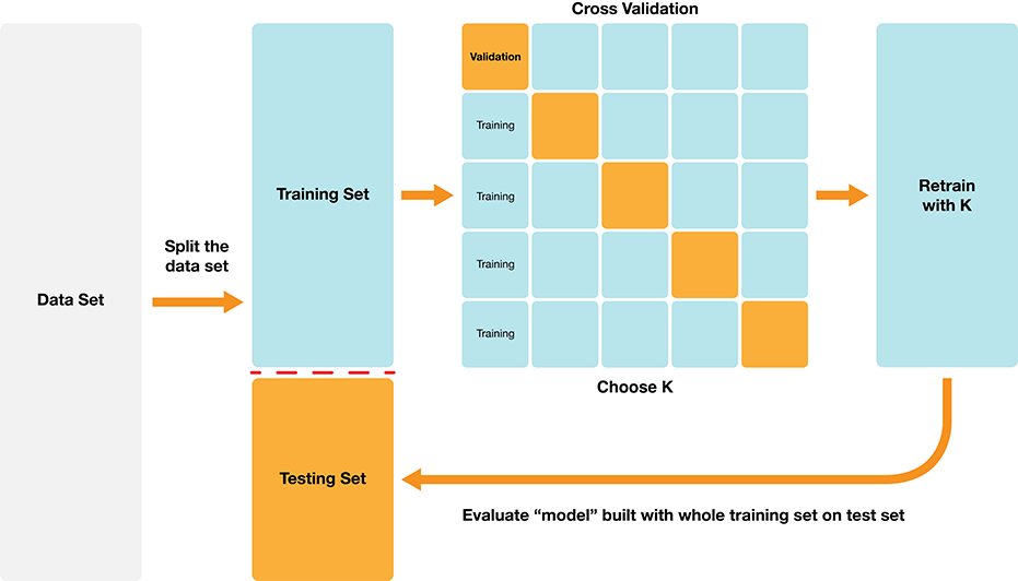
But we can split the training set into two partitions, a traning set and a validation set.
For each parameter value we want to assess, we can fit on the training set, and evaluate on the validation set.
Then after we find the best value for our parameter, we can refit the model with the best parameter on the entire training set and then evaluate our model on the test set.

Can we do better?

Depending on how we split the data into the training and validation sets, we might get a lucky split (or an unlucky one) that doesn’t give us a good estimate of the model’s true accuracy.
In many cases, we can do better by making many splits, and averaging the accuracy scores to get a better estimate.
We call this cross-validation.

Cross-validation

An example of 5-fold cross-validation:

Cross-validation in `scikit-learn`

Use the scikit-learn cross_validate function.
Need to specify:
- a modelling Pipeline as the estimator argument,
- the number of folds as the cv argument,
- the training data predictors as the X argument
- the labels as the y arguments.
Note that the cross_validate function handles stratifying the classes in each train and validate fold automatically.

from sklearn.model_selection import cross_validate

knn = KNeighborsClassifier(n_neighbors=3)
cancer_pipe = make_pipeline(cancer_preprocessor, knn)
X = cancer_train[["Smoothness", "Concavity"]]
y = cancer_train["Class"]
cv_10_df = pd.DataFrame(
    cross_validate(
        estimator=cancer_pipe,
        cv=10,
        X=X,
        y=y
    )
)

print(cv_10_df)

    fit_time  score_time  test_score
0   0.005057    0.007228    0.860465
1   0.004730    0.006983    0.837209
..       ...         ...         ...
8   0.003929    0.004518    0.904762
9   0.003947    0.004665    0.880952

[10 rows x 3 columns]

cv_10_metrics = cv_10_df.agg(["mean", "sem"])
cv_10_metrics['test_score']

mean    0.884939
sem     0.013360
Name: test_score, dtype: float64

Parameter value selection

Since cross-validation helps us evaluate the accuracy of our classifier, we can use cross-validation to calculate an accuracy for each value of our parameter, here \(K\), in a reasonable range,
Then we pick the value of \(K\) that gives us the best accuracy, and refit the model with our parameter on the training data, and then evaluate on the test data.
The scikit-learn package collection provides built-in functionality, named GridSearchCV, to automatically handle the details for us.

Parameter value selection

knn = KNeighborsClassifier() #don't specify the number of neighbours
cancer_tune_pipe = make_pipeline(cancer_preprocessor, knn)

parameter_grid = {
    "kneighborsclassifier__n_neighbors": range(1, 100, 5),
}

from sklearn.model_selection import GridSearchCV

cancer_tune_grid = GridSearchCV(
    estimator=cancer_tune_pipe,
    param_grid=parameter_grid,
    cv=10
)

Parameter value selection

Now we use the fit method on the GridSearchCV object to begin the tuning process.

cancer_tune_grid.fit(
    cancer_train[["Smoothness", "Concavity"]],
    cancer_train["Class"]
)
accuracies_grid = pd.DataFrame(cancer_tune_grid.cv_results_)
accuracies_grid.info()

<class 'pandas.core.frame.DataFrame'>
RangeIndex: 20 entries, 0 to 19
Data columns (total 19 columns):
 #   Column                                   Non-Null Count  Dtype  
---  ------                                   --------------  -----  
 0   mean_fit_time                            20 non-null     float64
 1   std_fit_time                             20 non-null     float64
 2   mean_score_time                          20 non-null     float64
 3   std_score_time                           20 non-null     float64
 4   param_kneighborsclassifier__n_neighbors  20 non-null     int64  
 5   params                                   20 non-null     object 
 6   split0_test_score                        20 non-null     float64
 7   split1_test_score                        20 non-null     float64
 8   split2_test_score                        20 non-null     float64
 9   split3_test_score                        20 non-null     float64
 10  split4_test_score                        20 non-null     float64
 11  split5_test_score                        20 non-null     float64
 12  split6_test_score                        20 non-null     float64
 13  split7_test_score                        20 non-null     float64
 14  split8_test_score                        20 non-null     float64
 15  split9_test_score                        20 non-null     float64
 16  mean_test_score                          20 non-null     float64
 17  std_test_score                           20 non-null     float64
 18  rank_test_score                          20 non-null     int32  
dtypes: float64(16), int32(1), int64(1), object(1)
memory usage: 3.0+ KB

Parameter value selection

accuracies_grid["sem_test_score"] = accuracies_grid["std_test_score"] / 10**(1/2)
accuracies_grid = (
    accuracies_grid[[
        "param_kneighborsclassifier__n_neighbors",
        "mean_test_score",
        "sem_test_score"
    ]]
    .rename(columns={"param_kneighborsclassifier__n_neighbors": "n_neighbors"})
)
print(accuracies_grid)

    n_neighbors  mean_test_score  sem_test_score
0             1         0.845127        0.019966
1             6         0.873200        0.015680
..          ...              ...             ...
18           91         0.875581        0.012967
19           96         0.875581        0.008193

[20 rows x 3 columns]

Visualize paramter value selection

accuracy_vs_k = (
    alt.Chart(accuracies_grid)
    .mark_line(point=True)
    .encode(
        x=alt.X("n_neighbors")
        .title("Neighbors"),
        y=alt.Y("mean_test_score")
        .scale(zero=False)
        .title("Accuracy estimate")
    )
)

Best parameter value

We can also obtain the number of neighbours with the highest accuracy programmatically by accessing the best_params_ attribute of the fit GridSearchCV object.

cancer_tune_grid.best_params_

{'kneighborsclassifier__n_neighbors': 36}

Best parameter value

Do we use \(K\) = 36?

Generally, when selecting a parameters, we are looking for a value where:

we get roughly optimal accuracy
changing the value to a nearby one doesn’t change the accuracy too much
the cost of training the model is not prohibitive

Under/Overfitting

What happens if we keep increasing the number of neighbors \(K\)?
The cross-validation accuracy estimate actually starts to decrease!

Evaluating on the test set

Before we evaluate on the test set, we need to refit the model using the best parameter(s) on the entire training set
Luckily, scikit-learn does it for us automatically!
To make predictions and assess the estimated accuracy of the best model on the test data, we can use the score and predict methods of the fit GridSearchCV object.

cancer_test["predicted"] = cancer_tune_grid.predict(
    cancer_test[["Smoothness", "Concavity"]]
)

Evaluating on the test set

We can then pass those predictions to the precision, recall, and crosstab functions to assess the estimated precision and recall, and print a confusion matrix.

cancer_tune_grid.score(
    cancer_test[["Smoothness", "Concavity"]],
    cancer_test["Class"]
)

0.9090909090909091

precision_score(
    y_true=cancer_test["Class"],
    y_pred=cancer_test["predicted"],
    pos_label='Malignant'
)

np.float64(0.8846153846153846)

recall_score(
    y_true=cancer_test["Class"],
    y_pred=cancer_test["predicted"],
    pos_label='Malignant'
)

np.float64(0.8679245283018868)

conf_matrix = pd.crosstab(
    cancer_test["Class"],
    cancer_test["predicted"]
)
print(conf_matrix)

predicted  Benign  Malignant
Class                       
Benign         84          6
Malignant       7         46

Summary

K-nearest neighbors classification algorithm

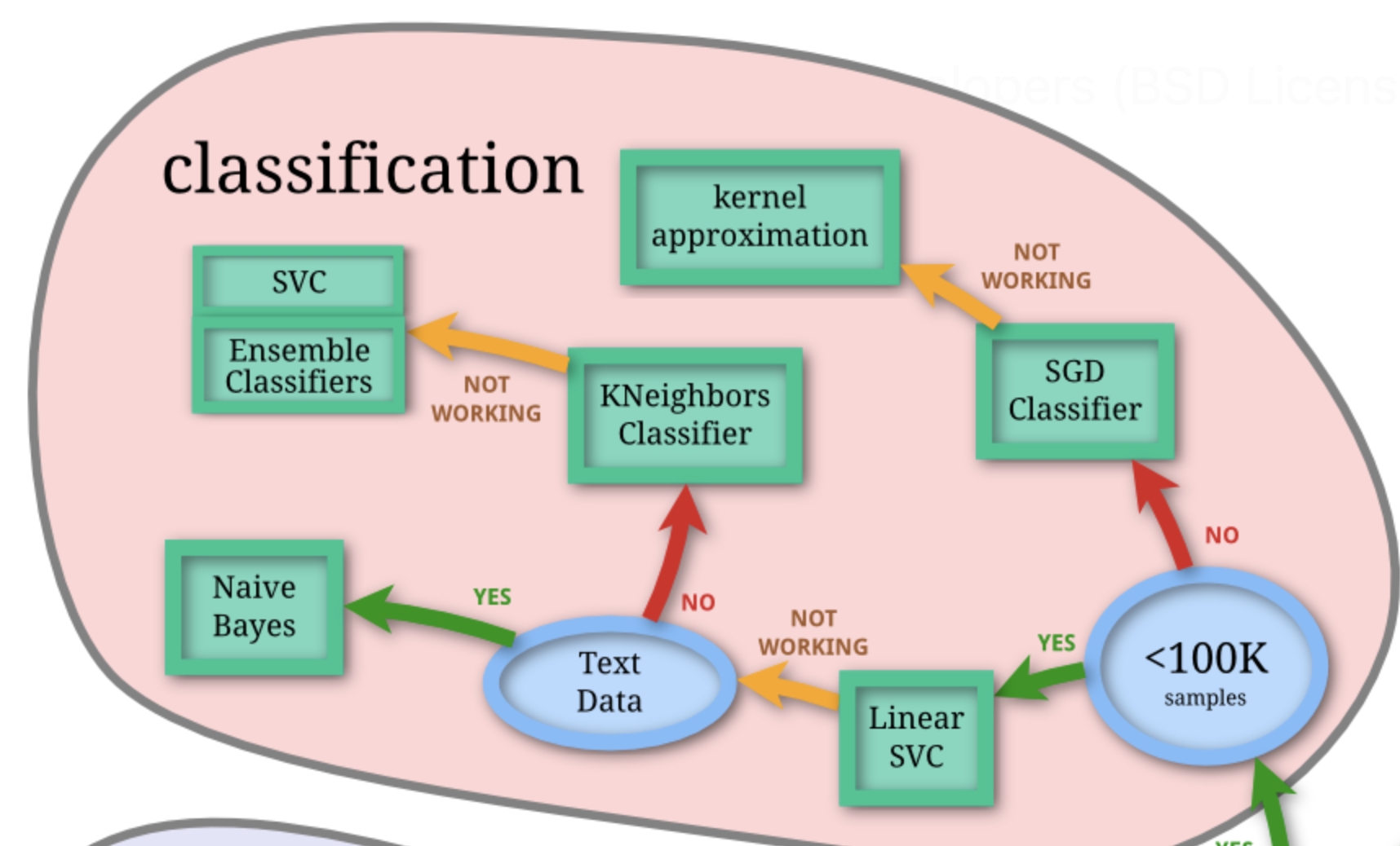
Strengths: K-nearest neighbors classification

is a simple, intuitive algorithm,
requires few assumptions about what the data must look like, and
works for binary (two-class) and multi-class (more than 2 classes) classification problems.

Weaknesses: K-nearest neighbors classification

becomes very slow as the training data gets larger,
may not perform well with a large number of predictors, and
may not perform well when classes are imbalanced.

Other classification algorithms

scikit-learn classification documentation: https://scikit-learn.org/stable/supervised_learning.html

Additional resources

The Classification II: evaluation & tuning chapter of Data Science: A First Introduction (Python Edition) by Tiffany Timbers, Trevor Campbell, Melissa Lee, Joel Ostblom, Lindsey Heagy contains all the content presented here with a detailed narrative.
The scikit-learn website is an excellent reference for more details on, and advanced usage of, the functions and packages in the past two chapters. Aside from that, it also offers many useful tutorials to get you started.
An Introduction to Statistical Learning {cite:p}james2013introduction provides a great next stop in the process of learning about classification. Chapter 4 discusses additional basic techniques for classification that we do not cover, such as logistic regression, linear discriminant analysis, and naive Bayes.

References

Evelyn Martin Lansdowne Beale, Maurice George Kendall, and David Mann. The discarding of variables in multivariate analysis. Biometrika, 54(3-4):357–366, 1967.

Norman Draper and Harry Smith. Applied Regression Analysis. Wiley, 1966.

M. Eforymson. Stepwise regression—a backward and forward look. In Eastern Regional Meetings of the Institute of Mathematical Statistics. 1966.

Ronald Hocking and R. N. Leslie. Selection of the best subset in regression analysis. Technometrics, 9(4):531–540, 1967.

Gareth James, Daniela Witten, Trevor Hastie, and Robert Tibshirani. An Introduction to Statistical Learning. Springer, 1st edition, 2013. URL: https://www.statlearning.com/.

Wes McKinney. Python for data analysis: Data wrangling with Pandas, NumPy, and IPython. ” O’Reilly Media, Inc.”, 2012.

William Nick Street, William Wolberg, and Olvi Mangasarian. Nuclear feature extraction for breast tumor diagnosis. In International Symposium on Electronic Imaging: Science and Technology. 1993.

Classification II: evaluation & tuning

Session learning objectives

Session learning objectives cont’d

Evaluating performance

Data splitting

Splitting the data into training and testing sets

Prediction accuracy

Is knowing accuracy enough?

Example confusion matrix for the breast cancer data:

Precision & recall

Precision and recall for the breast cancer data set example

Randomness and seeds

Setting the seed in Python

Setting the seed in Python (cont’d)

Back to the breast cancer data set example

Breast cancer data

Create the train / test split

Splitting the breast cancer data set

Checking the splits

Checking the splits

Preprocessing with data splitting

Preprocessing with scikit-learn

Train the classifier

Predict the labels in the test set

Evaluate performance

Accuracy, precision and recall

Confusion matrix

Critically analyze performance

Tuning the classifier

Validation set

Can we do better?

Cross-validation

Cross-validation in scikit-learn

Parameter value selection

Parameter value selection

Parameter value selection

Parameter value selection

Visualize paramter value selection

Best parameter value

Best parameter value

Under/Overfitting

Evaluating on the test set

Evaluating on the test set

Summary

K-nearest neighbors classification algorithm

Other classification algorithms

Additional resources

References

Preprocessing with `scikit-learn`

Cross-validation in `scikit-learn`