Introduction to machine learning in Python with Scikit-learn

Tree-based methods

Algorithms that stratifying or segmenting the predictor space into a number of simple regions.
We call these algorithms decision-tree methods because the decisions used to segment the predictor space can be summarized in a tree.
Decision trees on their own, are very explainable and intuitive, but not very powerful at predicting.
However, there are extensions of decision trees, such as random forest and boosted trees, which are very powerful at predicting. We will demonstrate two of these in this session.

Decision trees

Decision Trees by Jared Wilber & Lucía Santamaría

Classification Decision trees

Use recursive binary splitting to grow a classification tree (splitting of the predictor space into \(J\) distinct, non-overlapping regions).
For every observation that falls into the region \(R_j\) , we make the same prediction, which is the majority vote for the training observations in \(R_j\).
Where to split the predictor space is done in a top-down and greedy manner, and in practice for classification, the best split at any point in the algorithm is one that minimizes the Gini index (a measure of node purity).
Decision trees are useful because they are very interpretable.
A limitation of decision trees is that theyn tend to overfit, so in practice we use cross-validation to tune a hyperparameter, \(\alpha\), to find the optimal, pruned tree.

Example: the heart data set

Let’s consider a situation where we’d like to be able to predict the presence of heart disease (AHD) in patients, based off 13 measured characteristics.
The heart data set contains a binary outcome for heart disease for patients who presented with chest pain.

import pandas as pd
heart = pd.read_csv("data/Heart.csv", index_col=0)
heart.info()

<class 'pandas.core.frame.DataFrame'>
Index: 303 entries, 1 to 303
Data columns (total 14 columns):
 #   Column     Non-Null Count  Dtype  
---  ------     --------------  -----  
 0   Age        303 non-null    int64  
 1   Sex        303 non-null    int64  
 2   ChestPain  303 non-null    object 
 3   RestBP     303 non-null    int64  
 4   Chol       303 non-null    int64  
 5   Fbs        303 non-null    int64  
 6   RestECG    303 non-null    int64  
 7   MaxHR      303 non-null    int64  
 8   ExAng      303 non-null    int64  
 9   Oldpeak    303 non-null    float64
 10  Slope      303 non-null    int64  
 11  Ca         299 non-null    float64
 12  Thal       301 non-null    object 
 13  AHD        303 non-null    object 
dtypes: float64(2), int64(9), object(3)
memory usage: 35.5+ KB

Example: the heart data set

An angiographic test was performed and a label for AHD of Yes was labelled to indicate the presence of heart disease, otherwise the label was No.

heart.head()

	Age	Sex	ChestPain	RestBP	Chol	Fbs	RestECG	MaxHR	ExAng	Oldpeak	Slope	Ca	Thal	AHD
1	63	1	typical	145	233	1	2	150	0	2.3	3	0.0	fixed	No
2	67	1	asymptomatic	160	286	0	2	108	1	1.5	2	3.0	normal	Yes
3	67	1	asymptomatic	120	229	0	2	129	1	2.6	2	2.0	reversable	Yes
4	37	1	nonanginal	130	250	0	0	187	0	3.5	3	0.0	normal	No
5	41	0	nontypical	130	204	0	2	172	0	1.4	1	0.0	normal	No

Do we have a class imbalance?

It’s always important to check this, as it may impact your splitting and/or modeling decisions.

heart['AHD'].value_counts(normalize=True)

AHD
No     0.541254
Yes    0.458746
Name: proportion, dtype: float64

This looks pretty good! We can move forward this time without doing much more about this.

Data splitting

Let’s split the data into training and test sets:

import numpy as np
from sklearn.model_selection import train_test_split

np.random.seed(2024)

heart_train, heart_test = train_test_split(
    heart, train_size=0.8, stratify=heart["AHD"]
)

X_train = heart_train.drop(columns=['AHD'])
y_train = heart_train['AHD']
X_test = heart_test.drop(columns=['AHD'])
y_test = heart_test['AHD']

Categorical variables

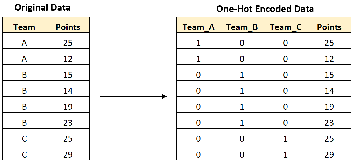
This is our first case of seeing categorical predictor variables, can we treat them the same as numerical ones? No!
In scikit-learn we must perform one-hot encoding

Source: https://scales.arabpsychology.com/stats/how-can-i-perform-one-hot-encoding-in-r/

Look at the data again

Which columns do we need to standardize?

Which do we need to one-hot encode?

heart.head()

	Age	Sex	ChestPain	RestBP	Chol	Fbs	RestECG	MaxHR	ExAng	Oldpeak	Slope	Ca	Thal	AHD
1	63	1	typical	145	233	1	2	150	0	2.3	3	0.0	fixed	No
2	67	1	asymptomatic	160	286	0	2	108	1	1.5	2	3.0	normal	Yes
3	67	1	asymptomatic	120	229	0	2	129	1	2.6	2	2.0	reversable	Yes
4	37	1	nonanginal	130	250	0	0	187	0	3.5	3	0.0	normal	No
5	41	0	nontypical	130	204	0	2	172	0	1.4	1	0.0	normal	No

One hot encoding & pre-processing

from sklearn.preprocessing import StandardScaler, OneHotEncoder
from sklearn.compose import make_column_transformer, make_column_selector

numeric_feats = ['Age', 'RestBP', 'Chol', 'RestECG', 'MaxHR', 'Oldpeak','Slope', 'Ca']
passthrough_feats = ['Sex', 'Fbs', 'ExAng']
categorical_feats = ['ChestPain', 'Thal']

heart_preprocessor = make_column_transformer(
    (StandardScaler(), numeric_feats),
    ("passthrough", passthrough_feats),
    (OneHotEncoder(handle_unknown = "ignore"), categorical_feats),
)

handle_unknown = "ignore" handles the case where categories exist in the test data, which were missing in the training set. Specifically, it sets the value for those to 0 for all cases of the category.

Fitting a dummy classifier

from sklearn.dummy import DummyClassifier
from sklearn.pipeline import make_pipeline
from sklearn.model_selection import cross_validate

dummy = DummyClassifier()
dummy_pipeline = make_pipeline(heart_preprocessor, dummy)
cv_10_dummy = pd.DataFrame(
    cross_validate(
        estimator=dummy_pipeline,
        cv=10,
        X=X_train,
        y=y_train
    )
)
cv_10_dummy_metrics = cv_10_dummy.agg(["mean", "sem"])
results = pd.DataFrame({'mean' : [cv_10_dummy_metrics.test_score.iloc[0]],
  'sem' : [cv_10_dummy_metrics.test_score.iloc[1]]},
  index = ['Dummy classifier']
)
results

	mean	sem
Dummy classifier	0.541333	0.00299

Fitting a decision tree

from sklearn.tree import DecisionTreeClassifier

decision_tree = DecisionTreeClassifier(random_state=2026)

dt_pipeline = make_pipeline(heart_preprocessor, decision_tree)
cv_10_dt = pd.DataFrame(
    cross_validate(
        estimator=dt_pipeline,
        cv=10,
        X=X_train,
        y=y_train
    )
)
cv_10_dt_metrics = cv_10_dt.agg(["mean", "sem"])
results_dt = pd.DataFrame({'mean' : [cv_10_dt_metrics.test_score.iloc[0]],
  'sem' : [cv_10_dt_metrics.test_score.iloc[1]]},
  index = ['Decision tree']
)
results = pd.concat([results, results_dt])
results

	mean	sem
Dummy classifier	0.541333	0.00299
Decision tree	0.769167	0.02632

Can we do better?

We could tune some decision tree parameters (e.g., alpha, maximum tree depth, etc)…
We could also try a different tree-based method!
The Random Forest Algorithm by Jenny Yeon & Jared Wilber

The Random Forest Algorithm

Build a number of decision trees on bootstrapped training samples.
When building the trees from the bootstrapped samples, at each stage of splitting, the best splitting is computed using a randomly selected subset of the features.
Take the majority votes across all the trees for the final prediction.

Random forest in `scikit-learn` & missing values

Does not accept missing values, we need to deal with these somehow…
We can either drop the observations with missing values, or we can somehow impute them.
For the purposes of this demo we will drop them, but if you are interested in imputation, see the imputation tutorial in scikit-learn

How many rows have missing observations:

heart.isna().any(axis=1).sum()

np.int64(6)

Drop rows with missing observations:

heart_train_drop_na = heart_train.dropna()

X_train_drop_na = heart_train_drop_na.drop(
    columns=['AHD']
)
y_train_drop_na = heart_train_drop_na['AHD']

Random forest in `scikit-learn`

from sklearn.ensemble import RandomForestClassifier

random_forest = RandomForestClassifier(random_state=2026)
rf_pipeline = make_pipeline(heart_preprocessor, random_forest)
cv_10_rf = pd.DataFrame(
    cross_validate(
        estimator=rf_pipeline,
        cv=10,
        X=X_train_drop_na,
        y=y_train_drop_na
    )
)

cv_10_rf_metrics = cv_10_rf.agg(["mean", "sem"])
results_rf = pd.DataFrame({'mean' : [cv_10_rf_metrics.test_score.iloc[0]],
  'sem' : [cv_10_rf_metrics.test_score.iloc[1]]},
  index = ['Random forest']
)
results = pd.concat([results, results_rf])
results

	mean	sem
Dummy classifier	0.541333	0.002990
Decision tree	0.769167	0.026320
Random forest	0.818297	0.017362

Can we do better?

Random forest can be tuned a several important parameters, including:
- n_estimators: number of decision trees (higher = more complexity)
- max_depth: max depth of each decision tree (higher = more complexity)
- max_features: the number of features you get to look at each split (higher = more complexity)
We can use GridSearchCV to search for the optimal parameters for these, as we did for \(K\) in \(K\)-nearest neighbors.

Tuning random forest in `scikit-learn`

from sklearn.model_selection import GridSearchCV

rf_param_grid = {'randomforestclassifier__n_estimators': [200],
              'randomforestclassifier__max_depth': [1, 3, 5, 7, 9],
              'randomforestclassifier__max_features': [1, 2, 3, 4, 5, 6, 7]}

rf_tune_grid = GridSearchCV(
    estimator=rf_pipeline,
    param_grid=rf_param_grid,
    cv=10,
    n_jobs=-1 # tells computer to use all available CPUs
)
rf_tune_grid.fit(
    X_train_drop_na,
    y_train_drop_na
)

cv_10_rf_tuned_metrics = pd.DataFrame(rf_tune_grid.cv_results_)
results_rf_tuned = pd.DataFrame({'mean' : rf_tune_grid.best_score_,
  'sem' : pd.DataFrame(rf_tune_grid.cv_results_)['std_test_score'][6] / 10**(1/2)},
  index = ['Random forest tuned']
)
results = pd.concat([results, results_rf_tuned])

Random Forest results

How did the Random Forest compare against the other models we tried?

results

	mean	sem
Dummy classifier	0.541333	0.002990
Decision tree	0.769167	0.026320
Random forest	0.818297	0.017362
Random forest tuned	0.860688	0.022223

Boosting

No randomization.
The key idea is combining many simple models called weak learners, to create a strong learner.
They combine multiple shallow (depth 1 to 5) decision trees.
They build trees in a serial manner, where each tree tries to correct the mistakes of the previous one.

Tuning `GradientBoostingClassifier` with `scikit-learn`

GradientBoostingClassifier can be tuned a several important parameters, including:
- n_estimators: number of decision trees (higher = more complexity)
- max_depth: max depth of each decision tree (higher = more complexity)
- learning_rate: the shrinkage parameter which controls the rate at which boosting learns. Values between 0.01 or 0.001 are typical.
We can use GridSearchCV to search for the optimal parameters for these, as we did for the parameters in Random Forest.

Tuning `GradientBoostingClassifier` with `scikit-learn`

from sklearn.ensemble import GradientBoostingClassifier

gradient_boosted_classifier = GradientBoostingClassifier(random_state=2026)
gb_pipeline = make_pipeline(heart_preprocessor, gradient_boosted_classifier)
gb_param_grid = {'gradientboostingclassifier__n_estimators': [200],
              'gradientboostingclassifier__max_depth': [1, 3, 5, 7, 9],
              'gradientboostingclassifier__learning_rate': [0.001, 0.005, 0.01]}
gb_tune_grid = GridSearchCV(
    estimator=gb_pipeline,
    param_grid=gb_param_grid,
    cv=10,
    n_jobs=-1 # tells computer to use all available CPUs
)
gb_tune_grid.fit(
    X_train_drop_na,
    y_train_drop_na
)

cv_10_gb_tuned_metrics = pd.DataFrame(gb_tune_grid.cv_results_)
results_gb_tuned = pd.DataFrame({'mean' : gb_tune_grid.best_score_,
  'sem' : pd.DataFrame(gb_tune_grid.cv_results_)['std_test_score'][6] / 10**(1/2)},
  index = ['Gradient boosted classifier tuned']
)
results = pd.concat([results, results_gb_tuned])

`GradientBoostingClassifier` results

How did the GradientBoostingClassifier compare against the other models we tried?

results

	mean	sem
Dummy classifier	0.541333	0.002990
Decision tree	0.769167	0.026320
Random forest	0.818297	0.017362
Random forest tuned	0.860688	0.022223
Gradient boosted classifier tuned	0.851993	0.025671

How do we choose the final model?

Remember, what is your question or application?
A good rule when models are not very different, what is the simplest model that does well?
Look at other metrics that are important to you (not just the metric you used for tuning your model), remember precision & recall, for example.
Remember - no peaking at the test set until you choose! And then, you should only look at the test set for one model!

Precision and recall on the tuned random forest model

from sklearn.metrics import make_scorer, precision_score, recall_score

scoring = {
    'accuracy': 'accuracy',
    'precision': make_scorer(precision_score, pos_label='Yes'),
    'recall': make_scorer(recall_score, pos_label='Yes')
}

rf_tune_grid = GridSearchCV(
    estimator=rf_pipeline,
    param_grid=rf_param_grid,
    cv=10,
    n_jobs=-1,
    scoring=scoring,
    refit='accuracy'
)

rf_tune_grid.fit(X_train_drop_na, y_train_drop_na)

Precision and recall cont’d

What do we think? Is this model ready for production in a diagnostic setting?
How could we improve it further?

cv_results = pd.DataFrame(rf_tune_grid.cv_results_)

mean_precision = cv_results['mean_test_precision'].iloc[rf_tune_grid.best_index_]
sem_precision = cv_results['std_test_precision'].iloc[rf_tune_grid.best_index_] / np.sqrt(10)
mean_recall = cv_results['mean_test_recall'].iloc[rf_tune_grid.best_index_]
sem_recall = cv_results['std_test_recall'].iloc[rf_tune_grid.best_index_] / np.sqrt(10)

results_rf_tuned = pd.DataFrame({
    'mean': [rf_tune_grid.best_score_, mean_precision, mean_recall],
    'sem': [cv_results['std_test_accuracy'].iloc[rf_tune_grid.best_index_] / np.sqrt(10), sem_precision, sem_recall],
}, index=['accuracy', 'precision', 'recall'])

results_rf_tuned

	mean	sem
accuracy	0.860688	0.018576
precision	0.920505	0.022982
recall	0.770909	0.038928

Feature importances

Key points:

Decision trees are very interpretable (decision rules!), however in ensemble models (e.g., Random Forest and Boosting) there are many trees - individual decision rules are not as meaningful…
Instead, we can calculate feature importances as the total decrease in impurity for all splits involving that feature, weighted by the number of samples involved in those splits, normalized and averaged over all the trees.
These are calculated on the training set, as that is the set the model is trained on.

Notes of caution!

Feature importances can be unreliable with both highly cardinal, and multicollinear features.
Unlike the linear model coefficients, feature importances do not have a sign! They tell us about importance, but not an “up or down”.
Increasing a feature may cause the prediction to first go up, and then go down.
Alternatives to feature importance to understanding models exist (e.g., SHAP (SHapley Additive exPlanations))

Feature importances in `scikit-learn`

# Access the best pipeline
best_pipeline = rf_tune_grid.best_estimator_

# Extract the trained RandomForestClassifier from the pipeline
best_rf = best_pipeline.named_steps['randomforestclassifier']

# Extract feature names after preprocessing
# Get the names of features from each transformer in the pipeline
numeric_features = numeric_feats
categorical_feature_names = best_pipeline.named_steps['columntransformer'].transformers_[2][1].get_feature_names_out(categorical_feats)
passthrough_features = passthrough_feats

# Combine all feature names into a single list
feature_names = np.concatenate([numeric_features, passthrough_features, categorical_feature_names])

# Calculate feature importances
feature_importances = best_rf.feature_importances_

# Create a DataFrame to display feature importances
importances_df = pd.DataFrame({
    'Feature': feature_names,
    'Importance': feature_importances
})

# Sort by importance (descending order)
importances_df = importances_df.sort_values(by='Importance', ascending=False)

Visualizing the results

Evaluating on the test set

Predict on the test set:

heart_test_drop_na = heart_test.dropna()
X_test_drop_na = heart_test_drop_na.drop(columns=['AHD'])
y_test_drop_na = heart_test_drop_na['AHD']

heart_test_drop_na["predicted"] = rf_tune_grid.predict(
    X_test_drop_na
)

Evaluating on the test set

Examine accuracy, precision and recall:

rf_tune_grid.score(
    X_test_drop_na,
    y_test_drop_na
)

0.7868852459016393

precision_score(
    y_true=heart_test_drop_na["AHD"],
    y_pred=heart_test_drop_na["predicted"],
    pos_label='Yes'
)

np.float64(0.8)

recall_score(
    y_true=heart_test_drop_na["AHD"],
    y_pred=heart_test_drop_na["predicted"],
    pos_label='Yes'
)

np.float64(0.7142857142857143)

conf_matrix = pd.crosstab(
    heart_test_drop_na["AHD"],
    heart_test_drop_na["predicted"]
)
print(conf_matrix)

predicted  No  Yes
AHD               
No         28    5
Yes         8   20

Other boosting models:

XGBoost

Not part of sklearn but has similar interface.
Supports missing values
GPU training, networked parallel training
Supports sparse data
Typically better scores than random forests

LightGBM

Not part of sklearn but has similar interface.
Small model size
Faster
Typically better scores than random forests

CatBoost

Not part of sklearn but has similar interface.
Usually better scores but slower compared to XGBoost and LightGBM

Keep learning!

https://python.datasciencebook.ca/

https://www.statlearning.com/

Local installation

Using Docker: Data Science: A First Introduction (Python Edition) Installation Instructions
Using conda: UBC MDS Installation Instructions

Additional resources

The UBC DSCI 573 (Feature and Model Selection notes) chapter of Data Science: A First Introduction (Python Edition) by Varada Kolhatkar and Joel Ostblom. These notes cover classification and regression metrics, advanced variable selection and more on ensembles.
The scikit-learn website is an excellent reference for more details on, and advanced usage of, the functions and packages in the past two chapters. Aside from that, it also offers many useful tutorials to get you started.
An Introduction to Statistical Learning {cite:p}james2013introduction provides a great next stop in the process of learning about classification. Chapter 4 discusses additional basic techniques for classification that we do not cover, such as logistic regression, linear discriminant analysis, and naive Bayes.

References

Gareth James, Daniela Witten, Trevor Hastie, Robert Tibshirani and Jonathan Taylor. An Introduction to Statistical Learning with Applications in Python. Springer, 1st edition, 2023. URL: https://www.statlearning.com/.

Kolhatkar, V., and Ostblom, J. (2024). UBC DSCI 573: Feature and Model Selection course notes. URL: https://ubc-mds.github.io/DSCI_573_feat-model-select

Pedregosa, F. et al., 2011. Scikit-learn: Machine learning in Python. Journal of machine learning research, 12(Oct), pp.2825–2830.

Tree-based and ensemble models

Tree-based methods

Decision trees

Classification Decision trees

Example: the heart data set

Example: the heart data set

Do we have a class imbalance?

Data splitting

Categorical variables

Look at the data again

One hot encoding & pre-processing

Fitting a dummy classifier

Fitting a decision tree

Can we do better?

The Random Forest Algorithm

Random forest in scikit-learn & missing values

Random forest in scikit-learn

Can we do better?

Tuning random forest in scikit-learn

Random Forest results

Boosting

Tuning GradientBoostingClassifier with scikit-learn

Tuning GradientBoostingClassifier with scikit-learn

GradientBoostingClassifier results

How do we choose the final model?

Precision and recall on the tuned random forest model

Precision and recall cont’d

Feature importances

Feature importances in scikit-learn

Visualizing the results

Evaluating on the test set

Evaluating on the test set

Other boosting models:

Keep learning!

Local installation

Additional resources

References

Random forest in `scikit-learn` & missing values

Random forest in `scikit-learn`

Tuning random forest in `scikit-learn`

Tuning `GradientBoostingClassifier` with `scikit-learn`

Tuning `GradientBoostingClassifier` with `scikit-learn`

`GradientBoostingClassifier` results

Feature importances in `scikit-learn`