useR to programmeR

Functions 2

Emma Rand and Ian Lyttle

Learning objectives

In this session, we will discuss:

• embracing {{}} for <data-masking> functions
• tidyverse style and design of functions
• the joys of side-effects

---

For coding, we will use r-programming-exercises:

• R/functions-02-01-embrace.R, etc.
• with each new file, restart R.

Plot functions: Motivation

library("tidyverse")

Sometimes, you want to generalize a certain type of plot - let’s say a histogram:

diamonds |> 
  ggplot(aes(x = carat)) +
  geom_histogram(binwidth = 0.1)

diamonds |> 
  ggplot(aes(x = carat)) +
  geom_histogram(binwidth = 0.05)

“I want choose only the data, variable, and bin-width”

Function

aes() is a data-masking function; you can embrace 🤗

• pass “bare-name” variables for data-frames
• look for <data-masking> in help

histogram <- function(df, var, binwidth = NULL) {
  df |> 
    ggplot(aes(x = {{ var }})) + 
    geom_histogram(binwidth = binwidth)
}

histogram(diamonds, carat, 0.1) 

Our turn

Complete this function yourself:

histogram <- function(df, var, binwidth = NULL) {
  df |>
    ggplot(aes()) +
    geom_histogram(binwidth = binwidth)
}

• Try with other df and var, e.g. starwars, mtcars.

• Using this function as is, how can you:

  • add theme_minimal()?

  • fill the bars with "steelblue"?

Our turn (solution)

Adding a theme: histogram() returns a ggplot object, so you can add a theme in the “usual” way:

histogram(starwars, height) + theme_minimal()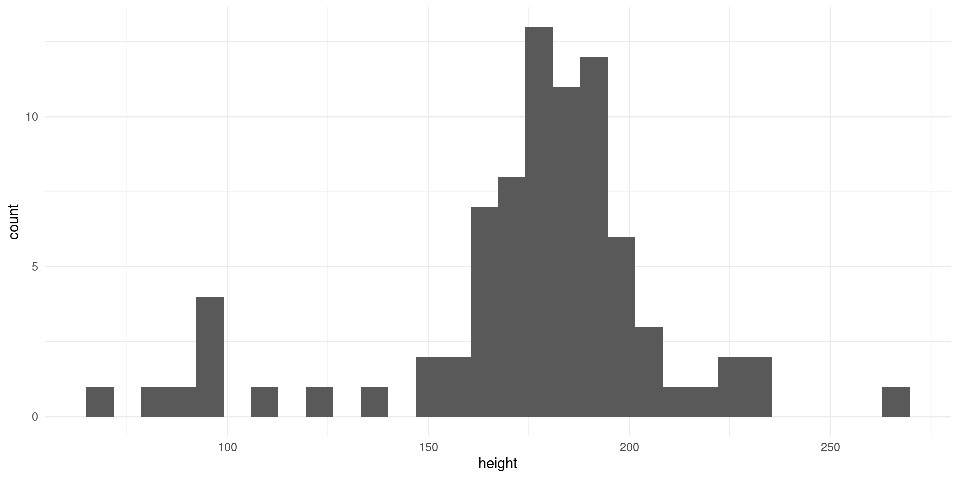

Our turn (solution)

As is, there is no easy way to specify "steelblue".

However, you can build an escape hatch.

... are called “dot-dot-dot” or “dots”.

# `...` passed to `geom_histogram()`
histogram <- function(df, var, ..., binwidth = NULL) {
  df |>
    ggplot(aes(x = {{var}})) +
    geom_histogram(binwidth = binwidth, ...)
}

Passes unspecified arguments from your function to another (tell your users where).

Tidyverse Design Guide has more details.

Our turn (continued)

Incorporate dot-dot-dot into histogram():

histogram <- function(df, var, ..., binwidth = NULL) {
  df |>
    ggplot(aes(x = {{var}})) +
    geom_histogram(binwidth = binwidth, ...)
}

Try, e.g.:

histogram(starwars, height, binwidth = 5, fill = "steelblue")

Tradeoffs

You write a function to make some things easier.

The cost is that some things become more difficult.

This is unavoidable, the best you can do is be deliberate about what you make easier and more difficult.

Labelling

How to build a string, using variable-names and values?

rlang::englue() was built for this purpose:

• embrace 🤗 variable-names: {{}}
• glue values: {}

temp <- function(varname, value) {
  rlang::englue("You chose varname: {{ varname }} and value: {value}")
}

temp(val, 0.4)

[1] "You chose varname: val and value: 0.4"

Your turn

Adapt histogram() to include a title that describes:

• which var is binned, and the binwidth

histogram <- function(df, var, ..., binwidth = NULL) {
  df |> 
    ggplot(aes(x = {{ var }})) + 
    geom_histogram(binwidth = binwidth, ...) + 
    labs(
      title = rlang::englue("")
    )
}

Try:

histogram(starwars, height, binwidth = 5)
histogram(starwars, height) # "extra credit"

Your turn (solution)

histogram <- function(df, var, ..., binwidth = NULL) {
  df |> 
    ggplot(aes(x = {{ var }})) + 
    geom_histogram(binwidth = binwidth, ...) + 
    labs(
      title = rlang::englue(
        "Histogram of {{ var }}, with binwidth {binwidth %||% 'default'}"
      )
    )
}

histogram(starwars, height, binwidth = 5)

Mixing in other tidyverse functions

Your function can also include pre-processing of data.

sorted_bars <- function(df, var) {
  df |> 
    mutate({{ var }} := {{ var }} |> fct_infreq() |> fct_rev()) |>
    ggplot(aes(y = {{ var }})) +
    geom_bar()
}

sorted_bars(diamonds, clarity)

Mixing in other tidyverse functions

Your function can also include pre-processing of data.

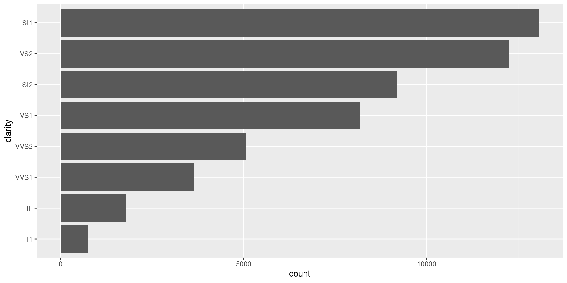
sorted_bars <- function(df, var) {
  df |> 
    mutate({{ var }} := {{ var }} |> fct_infreq() |> fct_rev()) |>
    ggplot(aes(y = {{ var }})) +
    geom_bar()
}

• If using { } to specify a new column, use :=, not =.

• fct_infreq() reorders by decreasing frequency.

• fct_rev() reverses order, as y-axis starts at bottom.

• Our turn: let’s try it

Summary (so far)

• use embracing {{}} to interpolate bare column-names

  • function receiving the “embracing” has to be aware
  • look for <data-masking> in the help
  • use rlang::englue() to interpolate variables {{}} and values {}

• ... is a useful “escape hatch” in function design:

  • put after required args, and before details
  • tell your users where the dots are going

Design and style

Restart R, open functions-02-02-style.R

---

Use descriptive name, usually starts with a verb, unless it returns a well-known noun.

mutate(): verb, describes what it does

median(): noun, describes what it returns

Order of arguments

• required: arguments without default values

• dots: can be passed on functions that your function calls

• optional: arguments with default values

Tidyverse Design:

• Position of dots

• Hadley’s first Substack article

Order of arguments

Our histogram function:

histogram <- function(df, var, ..., binwidth = NULL) {
  df |>
    ggplot(aes(x = {{var}})) +
    geom_histogram(binwidth = binwidth, ...)
}

• required: df, var

• dots: ...

• optional: binwidth

Order of arguments

histogram <- function(df, var, ..., binwidth = NULL) {
  df |> 
    ggplot(aes(x = {{ var }})) + 
    geom_histogram(binwidth = binwidth, ...) 
}

Why optional after dots?

• user must name optional arguments, in this case binwidth.

• makes code easier to read when optional arguments used.

• more reasoning given in the Tidyverse design guide.

Namespacing functions

When we write filter(), do we mean…

• dplyr::filter()?
• stats::filter()?

Three ways to sort this out:

• library("conflicted"), suitable for R scripts

• package::function(), used in package functions

• #' @importFrom, also used (sparingly) in packages

📦 conflicted

library("conflicted")

conflicted lets you know when you use a function that exists two-or-more packages that you’ve loaded.

To avoid conflicts, declare a preference:

# put in a conspicuous place, near the top of your script
conflicts_prefer(dplyr::filter)

Your turn

In functions-02-02-style.R:

library("tidyverse")

mtcars |> filter(cyl == 6)

• run it as-is
• add library("conflicted"), run again
• add a conflicts_prefer() directive

package::function()

This is the usual way when writing a function for a package:

histogram <- function(df, var, ..., binwidth = NULL) {
  df |> 
    ggplot2::ggplot(ggplot2::aes(x = {{ var }})) + 
    ggplot2::geom_histogram(binwidth = binwidth, ...) 
}

• makes it very clear where you are getting the function from
• can be verbose, especially if calling an external function often

There is a balance to be struck.

#' @importFrom

When you have a lot of calls to a given external function

Put this in {packagename}-package.R:

#' @importFrom ggplot2 ggplot aes geom_histogram
NULL

Alternatively, from the R command prompt:

usethis::use_import_from("ggplot2", c("ggplot", "aes", "geom_histogram"))

#' @importFrom

histogram <- function(df, var, ..., binwidth = NULL) {
  df |> 
    ggplot(aes(x = {{ var }})) + 
    geom_histogram(binwidth = binwidth, ...) 
}

Makes your code less verbose, but also less transparent

To mitigate:

• put all your @importFrom in one conspicuous file: {packagename}-package.R
• use judiciously

Design and style references

R for Data Science

Tidyverse Style Guide

Tidyverse Design Guide

Tidydesign Substack (Hadley)

Also, look at tidyverse code at GitHub (my favorite is {usethis})

Side effects

Restart R, open functions-02-03-side-effects.R

---

Pure function:

• Returns a value that depends only on its inputs, e.g. sum()

Uses side effects:

• Depends on something other than inputs, e.g. read.csv()

• Or, makes a change in the environment, e.g. print()

Pure function

add <- function(x, y) {
  x + y
}

The return value depends only on the inputs.

Easier to test.

Uses side effects

Side-effects can slow down your function:

• it can be costly to read/write to disk, print to the screen.

Depending on side effects can introduce uncertainty:

• are you certain of what file.csv contains?

Side effects aren’t necessarily bad, but you need to take them into account:

• need to take care when testing.

Your turn

Discuss with your neighbor, are these function-calls are pure, or do they use side effects?

In functions-02-03-side-effects.R:

x <- prod(1, 2, 3)

x <- print("Hello")

x <- ggplot(mtcars, aes(x = wt, y = mpg)) + geom_point()

x <- sort(c("apple", "Banana", "candle"))

Our turn: checking locale

Can be useful to consult devtools::session_info():

# using `info = "platform"` to fit output on screen
devtools::session_info(info = "platform")

─ Session info ───────────────────────────────────────────────────────────────
 setting  value
 version  R version 4.4.1 (2024-06-14)
 os       Ubuntu 22.04.4 LTS
 system   x86_64, linux-gnu
 ui       X11
 language (EN)
 collate  C.UTF-8
 ctype    C.UTF-8
 tz       UTC
 date     2024-08-11
 pandoc   3.2 @ /opt/quarto/bin/tools/ (via rmarkdown)

──────────────────────────────────────────────────────────────────────────────

Manage side effects using 📦 withr

Side effects can include:

• modifying environment: Sys.setenv()
• modifying options: options()
• setting random seed: set.seed()
• setting working directory: setwd()
• creating and writing to a temporary file

{withr} makes it a lot easier to “leave no footprints”.

Our turn: modifying locale

sort() uses locale (environment) for string-sorting rules

(temp <- Sys.getlocale("LC_COLLATE"))
## [1] "C.UTF-8"

sort(c("apple", "Banana", "candle"))
## [1] "apple"  "Banana" "candle"

---

Sys.setlocale("LC_COLLATE", "C")
## [1] "C"

sort(c("apple", "Banana", "candle"))
## [1] "Banana" "apple"  "candle"

Sys.setlocale("LC_COLLATE", temp)
## [1] "C.UTF-8"

Our turn: setting within call

To temporarily set locale:

withr::with_locale(
  new = list(LC_COLLATE = "C"),
  sort(c("apple", "Banana", "candle"))
)
## [1] "Banana" "apple"  "candle"

Sys.getlocale("LC_COLLATE")
## [1] "C.UTF-8"

Our turn: setting only within scope

c_sort <- function(...) {
  # set only within function block
  withr::local_locale(list(LC_COLLATE = "C"))
  
  sort(...)
}

c_sort(c("apple", "Banana", "candle"))
## [1] "Banana" "apple"  "candle"

Sys.getlocale("LC_COLLATE")
## [1] "C.UTF-8"

Within curly brackets applies to function blocks, it also applies to {testthat} blocks.

But what about dplyr?

• ?dplyr::arrange()
• arrange() uses the "C" locale by default

---

tibble(text = c("apple", "Banana", "candle")) |>
  arrange(text)

# A tibble: 3 × 1
  text  
  <chr> 
1 Banana
2 apple 
3 candle

Your turn

library("testthat")

test_that("mtcars has expected columns", {
  expect_type(mtcars$cy, "double")
})

Test passed 🥇

This passes, but R is doing partial matching on the $.

Modify test_that() block to warn on partial matching.

You can get the current setting using:

getOption("warnPartialMatchDollar")

[1] FALSE

Hint: use withr::local_option().

Your turn (solution)

test_that("mtcars has expected columns", {
  
  withr::local_options(list(warnPartialMatchDollar = TRUE))
  
  expect_type(mtcars$cy, "double")
})

── Warning: mtcars has expected columns ────────────────────────────────────────
partial match of 'cy' to 'cyl'
Backtrace:
    ▆
 1. └─testthat::expect_type(mtcars$cy, "double")
 2.   └─testthat::quasi_label(enquo(object), arg = "object")
 3.     └─rlang::eval_bare(expr, quo_get_env(quo))

And yet…

getOption("warnPartialMatchDollar")

[1] FALSE

Summary

You can use tidy evaluation in {ggplot2} to specify aesthetics, add labels, and include {dplyr} preprocessing:

• embracing {{}} for <data-masking> functions
• be aware of <tidy-select> functions, work differently

---

Using tidyverse style and design can make things easier for you, your users, and future you.

---

Be mindful of side effects, use {withr} to manage global state.