Parameters, interactivity,
and deployment
Build-a-Dashboard Workshop
2024-08-12
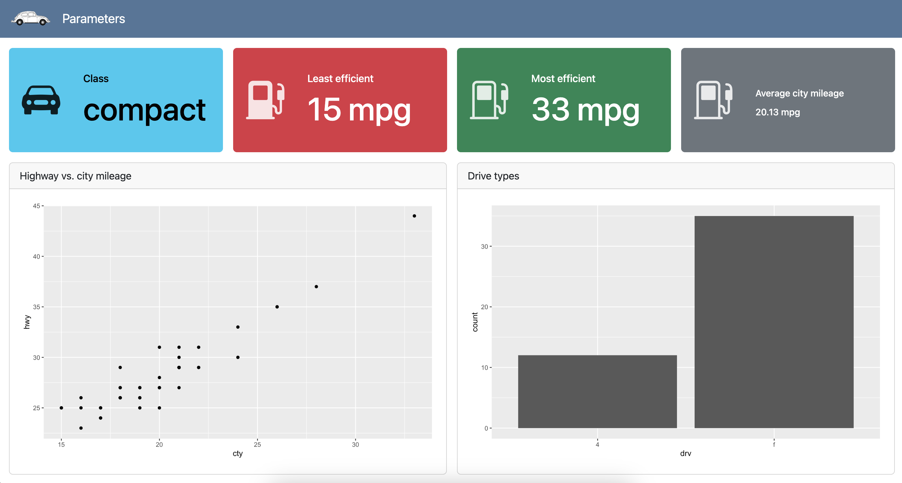
Parameters
dashboard-py.qmd
---
title: "Parameters"
format:
  dashboard:
    logo: images/beetle.png
params:
  class: "compact"
---

```{r}
library(ggplot2)
library(dplyr)
mpg <- mpg |>
  filter(class == params$class)
```

## Value boxes {height="25%"}

::: {.valuebox icon="car-front-fill" color="info"}
Class

`{r} params$class`
:::

```{r}
#| label: calculate-values
lowest_mileage_cty <- mpg |>
  filter(cty == min(cty)) |>
  distinct(cty) |>
  pull(cty)

highest_mileage_cty <- mpg |>
  filter(cty == max(cty)) |>
  distinct(cty) |>
  pull(cty)

rounded_mean_city_mileage <- mpg |>
  summarize(round(mean(cty), 2)) |>
  pull()
```

```{r}
#| content: valuebox
#| title: "Least efficient"
#| icon: fuel-pump-fill
#| color: danger
list(
  value = paste(lowest_mileage_cty, "mpg")
)
```

```{r}
#| content: valuebox
#| title: "Most efficient"
list(
  icon = "fuel-pump",
  color = "success",
  value = paste(highest_mileage_cty, "mpg")
)
```

::: {.valuebox icon="fuel-pump" color="secondary"}
Average city mileage

`{r} rounded_mean_city_mileage` mpg
:::

## Plots {height="75%"}

```{r}
#| title: Highway vs. city mileage
ggplot(mpg, aes(x = cty, y = hwy)) +
  geom_point()
```

```{r}
#| title: Drive types
ggplot(mpg, aes(x = drv)) +
  geom_bar()
```
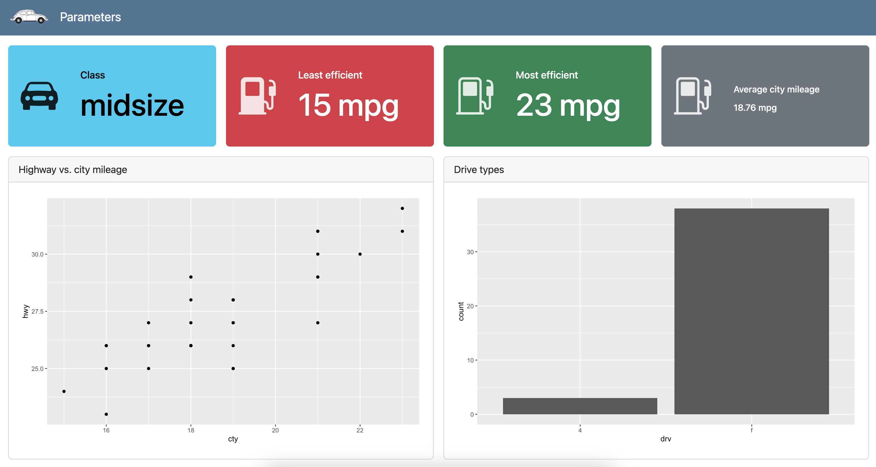
Parameters
dashboard-py.qmd
---
title: "Parameters"
format:
  dashboard:
    logo: images/beetle.png
params:
  class: "midsize"
---

```{r}
library(ggplot2)
library(dplyr)
mpg <- mpg |>
  filter(class == params$class)
```

## Value boxes {height="25%"}

::: {.valuebox icon="car-front-fill" color="info"}
Class

`{r} params$class`
:::

```{r}
#| label: calculate-values
lowest_mileage_cty <- mpg |>
  filter(cty == min(cty)) |>
  distinct(cty) |>
  pull(cty)

highest_mileage_cty <- mpg |>
  filter(cty == max(cty)) |>
  distinct(cty) |>
  pull(cty)

rounded_mean_city_mileage <- mpg |>
  summarize(round(mean(cty), 2)) |>
  pull()
```

```{r}
#| content: valuebox
#| title: "Least efficient"
#| icon: fuel-pump-fill
#| color: danger
list(
  value = paste(lowest_mileage_cty, "mpg")
)
```

```{r}
#| content: valuebox
#| title: "Most efficient"
list(
  icon = "fuel-pump",
  color = "success",
  value = paste(highest_mileage_cty, "mpg")
)
```

::: {.valuebox icon="fuel-pump" color="secondary"}
Average city mileage

`{r} rounded_mean_city_mileage` mpg
:::

## Plots {height="75%"}

```{r}
#| title: Highway vs. city mileage
ggplot(mpg, aes(x = cty, y = hwy)) +
  geom_point()
```

```{r}
#| title: Drive types
ggplot(mpg, aes(x = drv)) +
  geom_bar()
```
Thank you!
https://pos.it/conf-workshop-survey
![]()