7 Modeling

Catch up

library(sparklyr)
library(dplyr)
sc <- spark_connect(method = "databricks_connect")

7.1 Get sample of data

Download a sampled data set locally to R

Create a pointer to the lendingclub data. It is in the samples schema

lendingclub_dat <- tbl(sc, I("workshops.samples.lendingclub"))

Using slice_sample(), download 2K records, and name it lendingclub_sample

lendingclub_sample <- lendingclub_dat |>  
  slice_sample(n = 2000) |> 
  collect()

Preview the data using the View() command

View(lendingclub_sample)

Keep only int_rate, term, bc_util, bc_open_to_buy and all_util fields. Remove the percent sign out of int_rate, and coerce it to numeric. Save resulting table to a new variable called lendingclub_prep

lendingclub_prep <- lendingclub_sample |> 
  select(int_rate, term, bc_util, bc_open_to_buy, all_util) |> 
  mutate(
    int_rate = as.numeric(stringr::str_remove(int_rate, "%"))
    )

Preview the data using glimpse()

glimpse(lendingclub_prep)
#> Rows: 2,000
#> Columns: 5
#> $ int_rate       <dbl> 14.07, 12.61, 10.90, 9.58, 7.96, 5.31, 10.56, 18.45, 5.…
#> $ term           <chr> "36 months", "60 months", "36 months", "36 months", "36…
#> $ bc_util        <dbl> 8.5, 84.2, 95.4, 0.4, 16.6, 25.0, 28.3, 32.7, 53.6, 10.…
#> $ bc_open_to_buy <dbl> 21232, 835, 278, 20919, 37946, 41334, 17721, 64335, 343…
#> $ all_util       <dbl> 9, 61, 80, 61, 44, 29, 62, 33, 44, 19, 38, 37, 69, 29, …

Disconnect from Spark

spark_disconnect(sc)

7.2 Create model using `tidymodels`

Run the following code to create a workflow that contains the pre-processing steps, and a linear regression model

library(tidymodels)

lendingclub_rec <- recipe(int_rate ~ ., data = lendingclub_prep) |> 
  step_mutate(term = trimws(substr(term, 1,2))) |> 
  step_mutate(across(everything(), as.numeric)) |> 
  step_normalize(all_numeric_predictors()) |>
  step_impute_mean(all_of(c("bc_open_to_buy", "bc_util"))) |>   
  step_filter(!if_any(everything(), is.na))


lendingclub_lr <- linear_reg()

lendingclub_wf <- workflow() |> 
  add_model(lendingclub_lr) |> 
  add_recipe(lendingclub_rec)

lendingclub_wf
#> ══ Workflow ════════════════════════════════════════════════════════════════════
#> Preprocessor: Recipe
#> Model: linear_reg()
#> 
#> ── Preprocessor ────────────────────────────────────────────────────────────────
#> 5 Recipe Steps
#> 
#> • step_mutate()
#> • step_mutate()
#> • step_normalize()
#> • step_impute_mean()
#> • step_filter()
#> 
#> ── Model ───────────────────────────────────────────────────────────────────────
#> Linear Regression Model Specification (regression)
#> 
#> Computational engine: lm

Fit the model in the workflow, now in a variable called lendingclub_wf, with the lendingclub_prep data

lendingclub_fit <- lendingclub_wf |> 
  fit(data = lendingclub_prep)

Measure the performance of the model using metrics(). Make sure to use augment() to add the predictions first

lendingclub_fit |> 
  augment(lendingclub_prep) |> 
  metrics(int_rate, .pred)
#> # A tibble: 3 × 3
#>   .metric .estimator .estimate
#>   <chr>   <chr>          <dbl>
#> 1 rmse    standard       4.18 
#> 2 rsq     standard       0.307
#> 3 mae     standard       3.26

Run a histogram over the predictions

library(ggplot2)

predict(lendingclub_fit, lendingclub_sample) |> 
  ggplot() +
  geom_histogram(aes(.pred))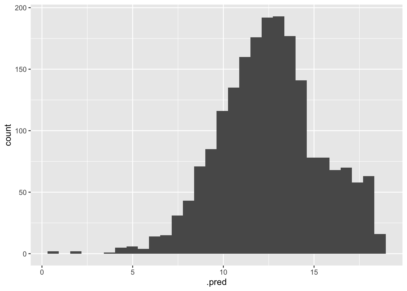

7.3 Using Vetiver

Convert the workflow into a vetiver model

Load the vetiver package

library(vetiver)

Convert to Vetiver using vetiver_model(). Name the variable lendingclub_vetiver

lendingclub_vetiver <- vetiver_model(lendingclub_fit, "lendingclub_model")

Save lendingclub_vetiver as “lendingclub.rds”

saveRDS(lendingclub_vetiver, "lendingclub.rds")

7.4 Create prediction function

Creating a self-contained prediction function that will read the model, and then run the predictions

Create a very simple function that takes x, and it assumes it will be a data frame. Inside the function, it will read the “lendingclub.rds” file, and then use it to predict against x. Name the function predict_vetiver

predict_vetiver <- function(x) {
  model <- readRDS("lendingclub.rds")  
  predict(model, x)
}

Test the predict_vetiver function against lendingclub_prep

predict_vetiver(lendingclub_prep)
#> # A tibble: 2,000 × 1
#>    .pred
#>    <dbl>
#>  1  8.35
#>  2 17.3 
#>  3 14.2 
#>  4 10.1 
#>  5  8.77
#>  6  8.22
#>  7 10.9 
#>  8  7.14
#>  9 11.8 
#> 10  8.00
#> # ℹ 1,990 more rows

Modify the function, so that it will add the predictions back to x. The new variable should be named ret_pred. The function should output the modified x

predict_vetiver <- function(x) {
  model <- readRDS("lendingclub.rds")  
  preds <- predict(model, x)
  x$rate_pred <- preds$`.pred`
  x
}

Test the predict_vetiver function against lendingclub_prep

predict_vetiver(lendingclub_prep)
#> # A tibble: 2,000 × 6
#>    int_rate term      bc_util bc_open_to_buy all_util rate_pred
#>       <dbl> <chr>       <dbl>          <dbl>    <dbl>     <dbl>
#>  1    14.1  36 months     8.5          21232        9      8.35
#>  2    12.6  60 months    84.2            835       61     17.3 
#>  3    10.9  36 months    95.4            278       80     14.2 
#>  4     9.58 36 months     0.4          20919       61     10.1 
#>  5     7.96 36 months    16.6          37946       44      8.77
#>  6     5.31 36 months    25            41334       29      8.22
#>  7    10.6  36 months    28.3          17721       62     10.9 
#>  8    18.4  36 months    32.7          64335       33      7.14
#>  9     5.31 36 months    53.6           3434       44     11.8 
#> 10     7.46 36 months    10.9          33668       19      8.00
#> # ℹ 1,990 more rows

At the beginning of the function, load the workflows and vetiver libraries

predict_vetiver <- function(x) {
  library(workflows)
  library(vetiver)
  model <- readRDS("lendingclub.rds")  
  preds <- predict(model, x)
  x$rate_pred <- preds$`.pred`
  x
}

Test the predict_vetiver function against lendingclub_prep

predict_vetiver(lendingclub_prep)
#> # A tibble: 2,000 × 6
#>    int_rate term      bc_util bc_open_to_buy all_util rate_pred
#>       <dbl> <chr>       <dbl>          <dbl>    <dbl>     <dbl>
#>  1    14.1  36 months     8.5          21232        9      8.35
#>  2    12.6  60 months    84.2            835       61     17.3 
#>  3    10.9  36 months    95.4            278       80     14.2 
#>  4     9.58 36 months     0.4          20919       61     10.1 
#>  5     7.96 36 months    16.6          37946       44      8.77
#>  6     5.31 36 months    25            41334       29      8.22
#>  7    10.6  36 months    28.3          17721       62     10.9 
#>  8    18.4  36 months    32.7          64335       33      7.14
#>  9     5.31 36 months    53.6           3434       44     11.8 
#> 10     7.46 36 months    10.9          33668       19      8.00
#> # ℹ 1,990 more rows

7.5 Predict in Spark

Run the predictions in Spark against the entire data set

Add conditional statement that reads the RDS file if it’s available locally, and if not, read it from: “/Volumes/workshops/models/vetiver/lendingclub.rds”

predict_vetiver <- function(x) {
  library(workflows)
  library(vetiver)
  if(file.exists("lendingclub.rds")) {
    model <- readRDS("lendingclub.rds")  
  } else {
    model <- readRDS("/Volumes/workshops/models/vetiver/lendingclub.rds")
  }
  preds <- predict(model, x)
  x$rate_pred <- preds$`.pred`
  x
}

Re-connect to your Spark cluster

sc <- spark_connect(method = "databricks_connect")

Re-create a pointer to the lendingclub data. It is in the samples schema

lendingclub_dat <- tbl(sc, I("workshops.samples.lendingclub"))

Select the int_rate, term, bc_util, bc_open_to_buy, and all_util fields from lendingclub_dat. And then pass just the top rows (using head()) to spark_apply(). Use the updated predict_vetiver to run the model.

lendingclub_dat |> 
  select(int_rate, term, bc_util, bc_open_to_buy, all_util) |> 
  head() |> 
  spark_apply(predict_vetiver)
#> # Source:   table<`sparklyr_tmp_table_ccf6db3c_0348_4246_8a93_765344c7f00a`> [6 x 6]
#> # Database: spark_connection
#>   int_rate term      bc_util bc_open_to_buy all_util rate_pred
#>   <chr>    <chr>       <dbl>          <dbl>    <dbl>     <dbl>
#> 1 20.39%   36 months    94              133       82     14.9 
#> 2 13.06%   60 months    82            10021       70     17.2 
#> 3 10.56%   60 months    34.5          41570       54     13.4 
#> 4 6.83%    36 months     7.9          23119       47      9.43
#> 5 17.47%   60 months    62.1          11686       57     16.0 
#> 6 16.46%   36 months    92.2            380       75     14.6

Add the columns specification to the spark_apply() call

lendingclub_dat |> 
  select(int_rate, term, bc_util, bc_open_to_buy, all_util) |> 
  head() |> 
  spark_apply(
    predict_vetiver, 
    columns = "int_rate string, term string, bc_util double, bc_open_to_buy double, all_util double, pred double"
    )
#> # Source:   table<`sparklyr_tmp_table_63178bba_c8ea_4f0b_aa19_c3377c947124`> [6 x 6]
#> # Database: spark_connection
#>   int_rate term      bc_util bc_open_to_buy all_util  pred
#>   <chr>    <chr>       <dbl>          <dbl>    <dbl> <dbl>
#> 1 20.39%   36 months    94              133       82 14.9 
#> 2 13.06%   60 months    82            10021       70 17.2 
#> 3 10.56%   60 months    34.5          41570       54 13.4 
#> 4 6.83%    36 months     7.9          23119       47  9.43
#> 5 17.47%   60 months    62.1          11686       57 16.0 
#> 6 16.46%   36 months    92.2            380       75 14.6

Append compute() to the end of the code, remove head(), and save the results into a variable called lendingclub_predictions

lendingclub_predictions <- lendingclub_dat |> 
  select(int_rate, term, bc_util, bc_open_to_buy, all_util) |> 
  spark_apply(
    predict_vetiver,
    columns = "int_rate string, term string, bc_util double, bc_open_to_buy double, all_util double, pred double"
    ) |> 
  compute()

Preview the lendingclub_predictions table

lendingclub_predictions
#> # Source:   table<`table_6ba184f8_9933_4bdd_88da_cc5f27fc4e91`> [?? x 6]
#> # Database: spark_connection
#>    int_rate term      bc_util bc_open_to_buy all_util  pred
#>    <chr>    <chr>       <dbl>          <dbl>    <dbl> <dbl>
#>  1 20.39%   36 months    94              133       82 14.9 
#>  2 13.06%   60 months    82            10021       70 17.2 
#>  3 10.56%   60 months    34.5          41570       54 13.4 
#>  4 6.83%    36 months     7.9          23119       47  9.43
#>  5 17.47%   60 months    62.1          11686       57 16.0 
#>  6 16.46%   36 months    92.2            380       75 14.6 
#>  7 19.42%   60 months    21.5           1099       12 13.5 
#>  8 22.90%   60 months    36.1          30777       62 14.3 
#>  9 5.31%    36 months    54.9           8576       71 12.7 
#> 10 6.83%    36 months    12.4          53356       17  6.96
#> # ℹ more rows